In this post, I take a look at the basic idea of why the logistic regression’s familiar S-curve exists, its relation to the familiar concept of probability, and how framing probability as the logarithm of odds naturally leads to a representation amenable to linear regression.
I returned to learning some classical machine learning recently, mostly to brush up on some of the foundational math. I usually do this in order to not let my brain rot from just applying language models to any task that presents itself. One of the earliest concepts I learnt in classical ML is Logistic Regression. For the longest time, I had a very simplistic, incomplete, and frankly wrong, idea of what LR was actually doing, what it represented, and why it worked. Ironically, the most understanding I gained was from conversing with Claude, forcing it to slow down, and clarify every misunderstanding in excruciating detail until I was convinced that I understood. Of course, mere understanding is not enough, so I’d like to document it, in the hopes that future me (who will have forgotten this material all over again) will find this a valuable aid to recollection.
Expressing probability as odds
We all know probability, right? That number between 0 and 1, or if you are feeling inclined towards percentages, between 0 and 100%; we use it to express, loosely, the likelihood of something happening (ignoring the fact for now, that likelihood has a very specific meaning in the subject). However, there is another way to express the chance of something happening, and that is by expressing odds. When someone says “What are the odds of it raining?”, let’s see what different answers could mean.
- I answer: “I give it even odds”, I’m saying that the probability of it raining is the same as it not raining.
- I answer: “I think the odds are 2 to 1 it is going to rain.”, I’m saying that the chance of it raining is double of that of it not raining.
Both of these can be expressed precisely. Assuming that rain and not rain are the only two possibilities:
For the first answer, we can write:
\[p_{rain} + p_{dry} = 1 \text{..............Probabilities sum to 1} \\ p_{rain} = p_{dry} \text{....................Odds are even}\\ \Rightarrow 2 \cdot p_{rain} = 1 \\ \Rightarrow p_{rain} = p_{dry} = 0.5\]For the second answer, we can write:
\[p_{rain} + p_{dry} = 1 \\ p_{rain} = 2 \cdot p_{dry} \\ \Rightarrow 2 \cdot p_{dry} + p_{dry} = 1 \\ \Rightarrow 3 \cdot p_{dry} = 1 \\ \Rightarrow p_{dry} = 0.33 \\ \Rightarrow p_{rain} = 0.67\]Thus, odds is the ratio of successful outcomes to unsuccessful outcomes, that is:
\[\text{odds(success)} = \frac {\text{successful outcomes}}{\text{unsuccessful outcomes}}\]Why is this useful? Because there is an important property of odds which the plain expression of probability does not have: odds can be any number between 0 and \(\infty\). An example will suffice. Suppose we say that the odds of it raining are some ridiculously large number, say one million to one. That means that:
\[p_{rain} + p_{dry} = 1 \\ p_{rain} = 10^6 \cdot p_{dry} \\ \Rightarrow 10^6 \cdot p_{dry} + p_{dry} = 1 \\ \Rightarrow 1000001 \cdot p_{dry} = 1 \\ \Rightarrow p_{dry} = 0.000000999999 \\ \Rightarrow p_{rain} = 0.999999\]So the probability of it not raining is very very small, but never zero, even in the presence of arbitrarily large numbers.
This is useful because it lets us express probabilities using arbitrary positive numbers. But the story is not over yet: we’d like to express probabilities using the entire number line, and this includes negative numbers. That’s the subject of the next section.
Expressing probability as log odds
There is a very simple way to jump from expressing probabilities using only positive numbers (using the language of odds) to include negative numbers: simply take the logarithm of odds. Take the example of “The odds of it raining are 1 to 3”. This is saying that it is thrice as likely to not rain as it is to rain. Note that the ratio now looks like:
\[\frac {p_{rain}}{p_{dry}} = \frac {1}{3} \\ odds_{rain} = \frac {1}{3}\]Now see what happens when we take log of these odds:
\[\ln(odds_{rain}) = - \ln(3) = −1.099\]The practical upshot is that if we choose to use log odds to express probabilities, we can express probabilities using the complete real number line.
If you are familiar with Generalised Linear Models, log odds is the link function.
The curve is the relationship between “normal” probability and log odds
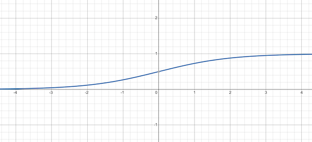
The fun part - and the point of this exercise - is to see what the original probability variable looks like when expressed in terms of log odds. This is a simple mathematical derivation which nevertheless reveals the S shape that we associate with the logistic regression curve.
Let \(t\) represent the log odds variable. Then we have:
\[t = \ln \frac {p}{1 - p} \\ \Rightarrow e^t = \frac {p}{1-p} \\ \Rightarrow e^t (1 - p) = p \\ \Rightarrow p (1 + e^t) = e^t \\ \Rightarrow p = \frac {e^t}{1 + e^t}\]Then we tidy up by dividing both numerator and denominator by \(e^t\) to get:
\[p = \frac {1}{1 + e^{-t}}\]That is the S-curve of logistic regression.
Regression on log odds
The reason we like the log odds representation is this: when we perform regression on the points to make the S-curve fit to them, we need a model of how the tuning parameters affect the curve. We’d like to have those tuning parameters represent a linear model, without the co-domain of the linear model being restricted to being between 0 and 1. The fitness function of the regression still measures the fit of the S-curve equation to the data.