Matrix Outer Product: Linear Combinations of Vectors

Avishek Sen Gupta on 30 March 2021

---

Matrix multiplication (outer product) is a fundamental operation in almost any Machine Learning proof, statement, or computation. Much insight may be gleaned by looking at different ways of looking matrix multiplication. In this post, we will look at one (and possibly the most important) interpretation: namely, the linear combination of vectors.

In fact, the geometric interpretation of this operation allows us to infer many properties that might be obscured if we were treating matrix multiplication as simple sums of products of numbers.

Quick Aside: There are some other ways of viewing matrix multiplication, which we will address in one of the future articles (element-wise, columns-into-rows).

To begin with, I’ll state the one fact that holds true no matter how you performing matrix multiplication. Even if you forget everything you read in this article, remember this thing:

Matrix multiplication is a linear combination of a set of vectors.

Let’s begin with a simple two-dimensional vector, like so: \(A_1=\begin{bmatrix} 2 \\ 3 \\ \end{bmatrix}\)

Let’s introduce a \(1\times 1\) vector \(x_1=\begin{bmatrix} 2 \\ \end{bmatrix}\)

We multiply them together, like so: \(Y=A_1x_1 = \begin{bmatrix} 2 \\ 3 \\ \end{bmatrix}.\begin{bmatrix} 2 \\ \end{bmatrix} =\begin{bmatrix} 4 \\ 6 \\ \end{bmatrix}\)

This is nothing special, simply a scaling of the \(\begin{bmatrix}2 && 3\end{bmatrix}^T\) matrix.

1. Linear Combination of Column Vectors

Let’s take the next step. We will add one more column vector to A, and add a number to \(x_1\).

\[A_2=\begin{bmatrix} 2 && 5\\ 3 && 10\\ \end{bmatrix} v_2=\begin{bmatrix} 2 \\ 3 \\ \end{bmatrix}\]

In this approach, we are only correlating columns on both sides. Consider the following diagram to see how this combination works.

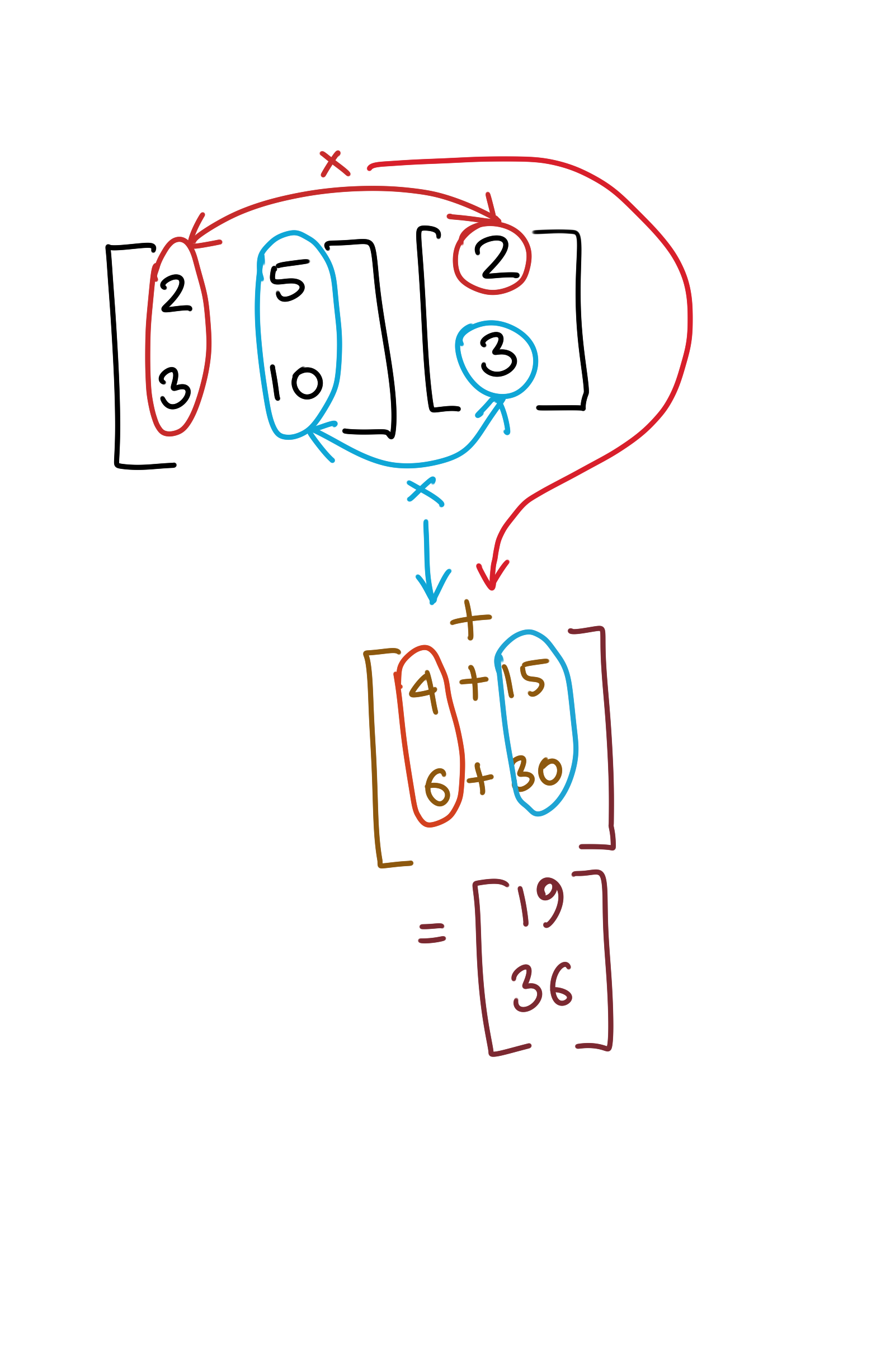
What you are really doing is this: you are considering the weighted sum of all the column vectors of \(A_2\) (Remember, in this picture, \(A_2\) is just a bunch of column vectors).

What are these weights? Each value in the column in \(v_2\) is a weight. Each weight scales a column vector, and these weighted vectors are added together to form a single column.

I hope it becomes obvious that this implies that the number of column vectors in \(A_2\) (the number of columns in \(A_2\)) must equal the number of values in \(v_2\)’s column (the number of rows in \(v_2\)), because there has to exist a one-to-one correspondence between them in order for this operation to be possible.

This results in a linear combination of the column vectors in \(A_2\). A linear combination of two vectors is of the form \(\alpha x + \beta y\), where \(\alpha\) and \(\beta\) are simple scalars (numbers). What you are really doing is either squashing or stretching some vectors by some factor (this can be a negative number), and then adding them together. That’s what a linear combination essentially means.

To put it more concretely in this example, your computation is as follows:

\[A_2=\left[2.\begin{bmatrix} 2 \\ 3 \\ \end{bmatrix} + 3.\begin{bmatrix} 5 \\ 10 \\ \end{bmatrix}\right]= \begin{bmatrix} 19 \\ 36 \\ \end{bmatrix}\]

1.1 The Geometric Interpretation

It is worth pausing to ground our understanding using the geometric interpretation. If you have followed the verbal explanation so far, the geometric interpretation should be pretty straightforward to comprehend.

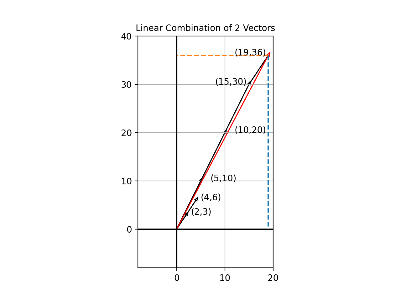
The vector \(\begin{bmatrix}2 && 3\end{bmatrix}^T\) is stretched by a factor of 2, to become \(\begin{bmatrix}4 && 6\end{bmatrix}^T\). Similarly, the vector \(\begin{bmatrix}5 && 10\end{bmatrix}^T\) is stretched by a factor of 3, to become \(\begin{bmatrix}15 && 30\end{bmatrix}^T\). The sum of these vectors is \(\begin{bmatrix}19 && 36\end{bmatrix}^T\), as indicated by the red arrow in the diagram above. This linear combination, as usual, extends to higher-dimensional vectors.

1.2 General Case

Let’s extend to the more general case, where we add another column to \(v_2\), so now that we have:

\[A_3=\begin{bmatrix} 2 && 5\\ 3 && 10\\ \end{bmatrix} v_3=\begin{bmatrix} 2 & -2\\ 3 & -4\\ \end{bmatrix}\]

How do we extend what we already know to this new case? Very simple: each column in \(v_3\) results in a corresponding column in the final result, and each output column is computed exactly the same. You are still linearly combining all the column vectors in \(A_3\), but the set of weights you’re using depends upon which column of \(v_3\) you are using for computation. Thus, this new computation is as follows:

\[A_2=\left[\left(2.\begin{bmatrix} 2 \\ 3 \\ \end{bmatrix} + 3.\begin{bmatrix} 5 \\ 10 \\ \end{bmatrix}\right) \left(-2.\begin{bmatrix} 2 \\ 3 \\ \end{bmatrix} + (-4).\begin{bmatrix} 5 \\ 10 \\ \end{bmatrix}\right)\right] \\ =\begin{bmatrix} 19 && -24\\ 36 && -46\\ \end{bmatrix}\]

Quick Aside: The column vectors which are linearly combined, come from the left side of the expression. The weights come from the right side. This is important to know, since the row column interpretation (which we will study next) inverts the order.

2. Linear Combination of Row Vectors

The concept of linear combination of vectors works equally well, if you consider the rows of a matrix as vectors. The same concept applies: each row in the output is the sum of all the weighted row vectors.

There is one important distinction, however, which is worth noting. In the column vector approach, the column vectors are on the left of the expression, which is to say, the expression is of the form \(Av\).

In the row vector approach, if you want to consider the rows as vectors, these vectors will come from the right hand side of the expression. Thus, if we wanted to perform the same operation, assuming we wish to use the same vectors, but treat them using the row vector approach, your expression has to assume the form \(v^TA^T\).

The algorithmic picture for multiplication using the row vector approach looks like this:

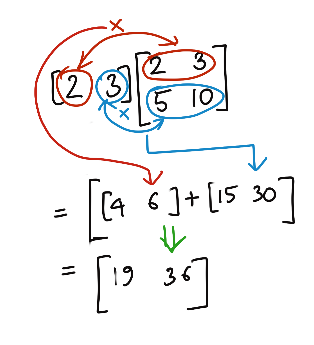
It is important to note that the central idea here (regardless of whether we are considering column vectors or row vectors) is that we are computing linear combinations of vectors. The geometric interpretation for this example stays the same. You should also convince yourself by doing this calculation by hand.

It is worth computing the original \(Av\) computation using the row vector approach, just to consider how different the rows are, and what the weights are. You should still get the same answer, however.

3. The Transponse of Matrix Multiplication

One thing you will have noticed is the way I set up the column vector and row vector examples.

Column Vector example: The computation was \(Av\) and the result was \(Y_1=\begin{bmatrix} 19 \\ 36 \\ \end{bmatrix}\) Row Vector example: The computation was \(v^TA^T\) and the result was \(Y_2=\begin{bmatrix} 19 && 36 \\ \end{bmatrix}\)

Obviously, \(Y_1^T=Y_2\). Substituting the original expressions in the above, we get:

\[(Av)^T=v^TA^T\]

This is just an example, but it is part of a more general rule about transposes, which is that:

The transpose of a set of operations is the same set of operations on the transposed elements, but applied in reverse order. We will sketch out a simple proof for this when we look at another method of matrix multiplication in one of the next articles.

We will also see a similar rule for inverses when discussing inverse matrices.

Conclusion

• The fact that columns (and rows) of the product of matrices can be treated as a linear combinations of vectors, is the important idea behind the Gaussian (and the Gauss-Jordan) Elimination method for solving systems of equations, which is very related to how students solve simultaneous equations in high school algebra.
• This insight also has important implications for the vector subspace that the resulting product matrix spans, as well as its rank, which we will talk about in future articles.

---