Linear Regression: Assumptions and Results using the Maximum Likelihood Estimator

Avishek Sen Gupta on 5 April 2021

---

Let’s look at Linear Regression. The “linear” term refers to the fact that the output variable is a linear combination of the input variables.

Thus, this is a linear equation:

\[y=ax_1+bx_2+cx_3\]

but this next ones are not:

\[y=ax_1+bx_2x_3+cx_3 \\ y=ax_1+bx_2+cx_3{x_1}^2\]

In the general form, we are looking for a relation like:

\[\mathbf{ y=w_1x_1+w_2x_2+...+w_Nx_N \\ y=\sum_{i=1}^Nw_ix_i }\]

Linear regression is a useful (and uncomplicated) tool for building prediction models, either on its own, or in its more sophisticated incarnations (like General Linear Models or Piecewise Linear Regression). However, it is instructive to consider the applicability of the linear model in its simplest form to a set of data, because there are very specific guarantees that the data should provide if we are to represent it using a linear model.

We will state these assumptions, as well as derive them from the base assumptions; some pictures should also clarify the intuition behind these intuitions. Parts of this will require a basic understanding of what probability distributions and partial differential calculus to follow along, but not much beyond that.

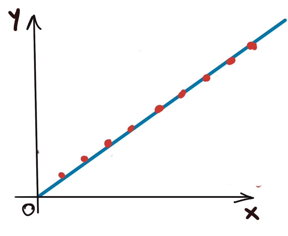
Let’s develop some intuition first through some examples. Check the diagram below. It should be obvious that this dataset can be modelled using linear regression. What this demonstrates specifically though, is the linear relationship between the input and the output, if we discount all other factors.

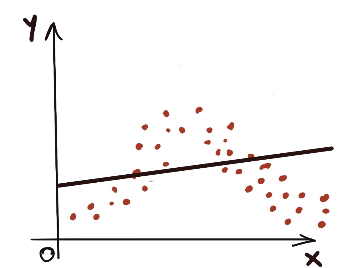
In contrast, the following picture demonstrates a clearly nonlinear relationship between the input and the output data.

Let’s go back to the simple perfectly fit data set above. Obviously, no data set is going to be perfect like the contrived example above, so you are more likely to see data like this:

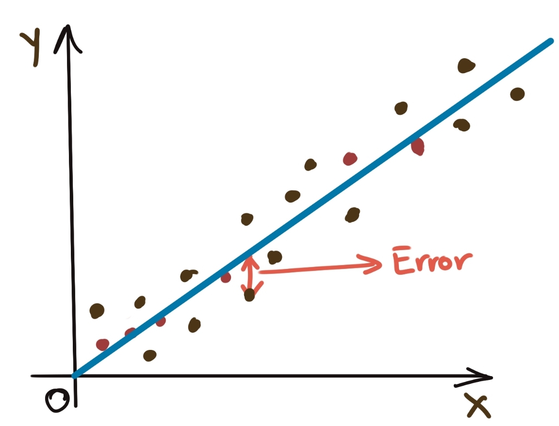
Thus, the prediction will never perfectly match the data (if it did, we have another problem, called overfitting, which we will visit sometime), but perfect prediction is not really the aim here, because observations can be easily affected by noise and other random effects. However, the effect of the noise needs to be quantified in some fashion, even if we cannot make accurate pointwise predictions about what the noise/error effect for a particular observation can be.

As it turns out, this leads us to the second important assumption about modelling data using Linear Regression, namely:

The noise/error values are normally distributed around the prediction.

Put another way, the error values should be equally randomly distributed around the prediction value. In terms of probability, this implies that the noise values should follow a Gaussian probability distribution. This also implies that we can assume that the prediction for a particular input is the average value of all the data points for that input (assuming multiple readings are taken for the same input). The prediction takes up the role of the mean in the resulting (hopefully) Gaussian distribution.

Let’s take the third example. Here, we definitely see a linear relationship between the input and output. The noise is also randomly distributed around the predicted value. But something else is going on here.

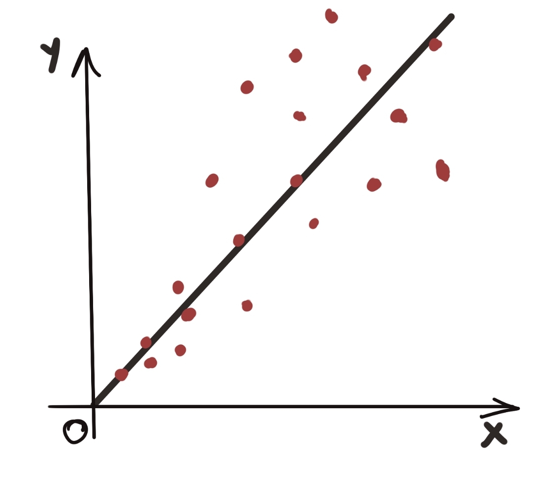
The graph tells us that even though the noise is normally distributed around the predicted value, the spread of these noise values is not constant. This leads us to the next important assumption of linear regression, namely that:

The noise values shouls be distributed with constant variance.

This above assumption could be folded into the linearity assumption, but I feel it is important enough to be stated on its own.

All of these assumptions can be summarised in the diagram below:

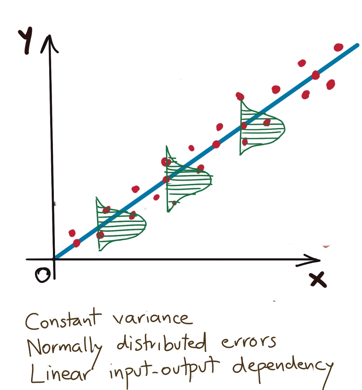
This shows that at each output value predicted by the model, the data is normally distributed with constant variance and the mean as the predicted value.

We would like to get a closed-form expression for the values of the mean and variance for a particular set of observations for a single value of input variable. That is, we want to estimate the parameters of the Gaussian distribution. In doing so, we want to ground our intuition of the mean being the average of N values from the Gaussian distribution assumption.

How do we approach this? To start from basic principles, we need to start with a probability approach. Let’s look at a couple of variations of the Gaussian distribution, one plot with varying means, the other with varying variance.

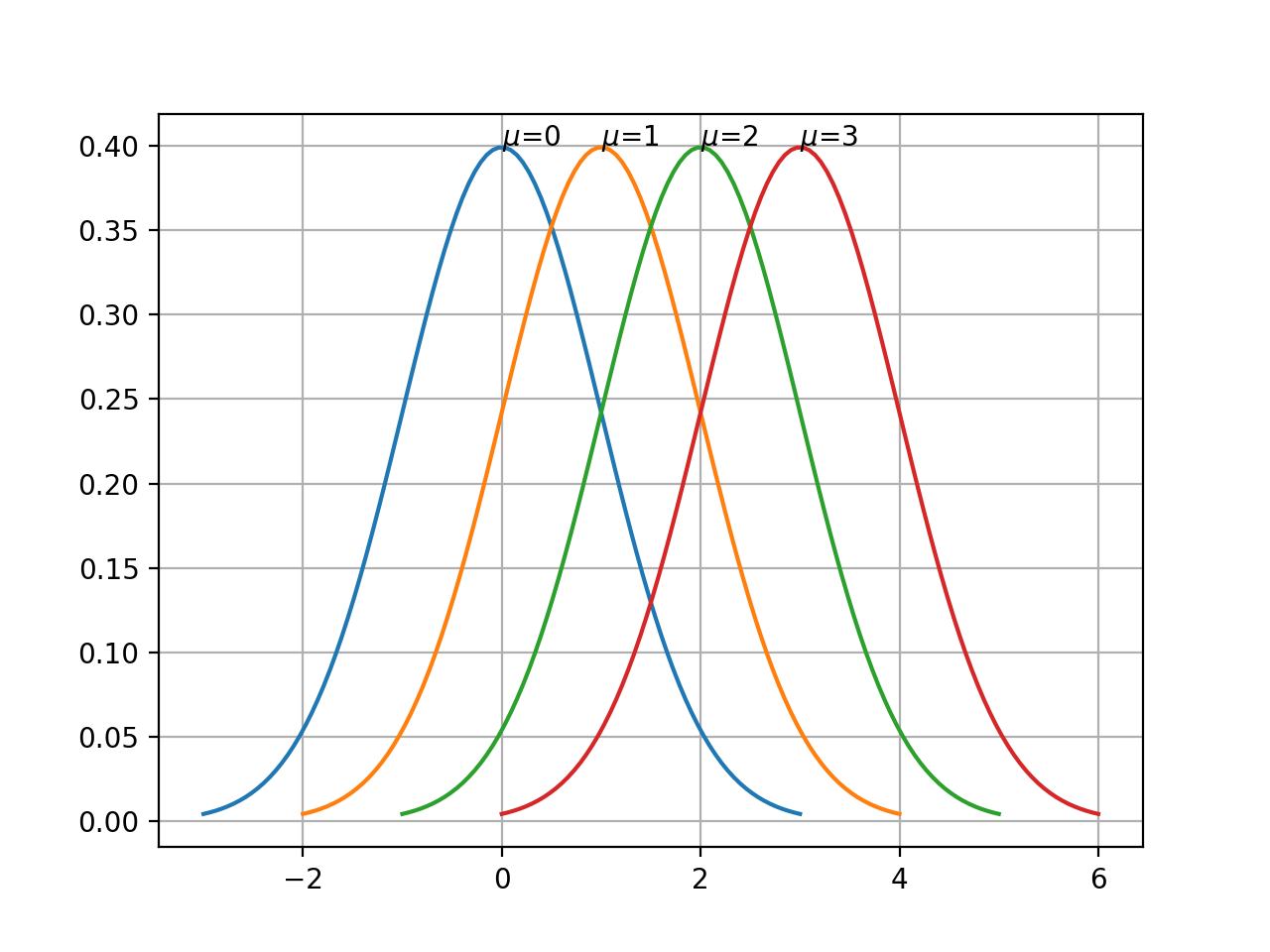
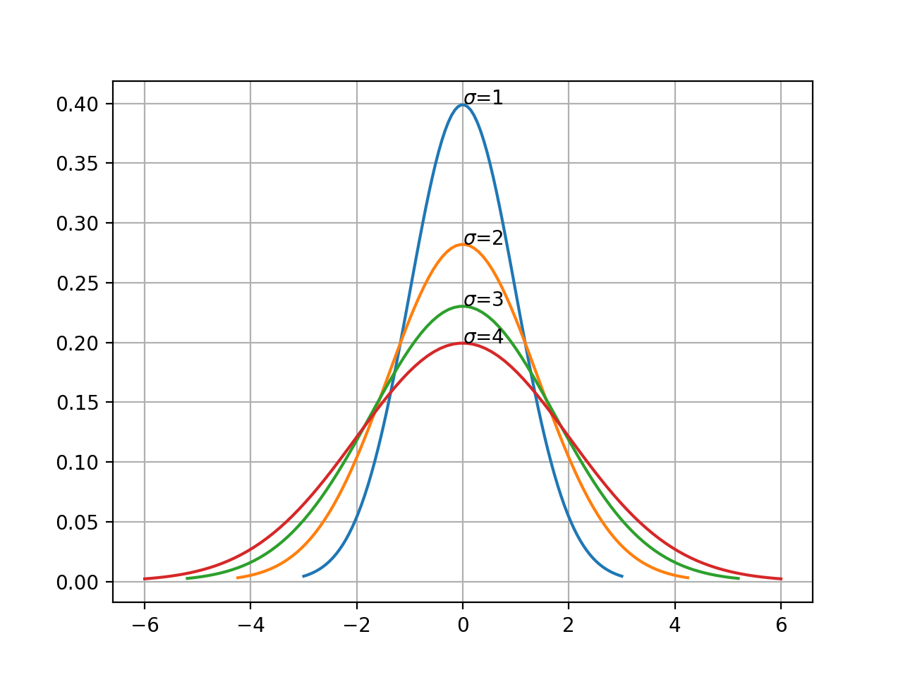
This yields different Gaussians depending on how we tune the parameters \(\mu\) and \(\sigma\). Our aim is to find a combination of \((\mu, \sigma)\) which best explains the distribution of the observations for a particular input value.

Let us introduce the Gaussian probability density function. \(P(x)=\frac{1}{\sqrt{2\pi\sigma^2}}.e^{-\frac{ {(x-\mu)}^2}{2\sigma^2}}\)

Let us assume that for a given input I, we have a set of observations \((x_1, x_2, x_3,...,x_N)\).

Thus if we randomly pick a combination of \((\mu, \sigma)\), we can ask the question:

What is the probability of observation \(x_i\) occurring, given a parameter set \((\mu, \sigma)\)? For \(x_1\), \(x_2\), etc., this is obviously given by:

\[P(x_1)=\frac{1}{\sqrt{2\pi\sigma^2}}.e^{-\frac{ {(x_1-\mu)}^2}{2\sigma^2}} \\ P(x_2)=\frac{1}{\sqrt{2\pi\sigma^2}}.e^{-\frac{ {(x_2-\mu)}^2}{2\sigma^2}} \\ .\\ .\\ .\\ P(x_N)=\frac{1}{\sqrt{2\pi\sigma^2}}.e^{-\frac{ {(x_N-\mu)}^2}{2\sigma^2}}\]

Knowing this, we can say that the joint probability of all the observations \((x_1, x_2, x_3,...,x_N)\) occurring for a given parameter set \((\mu, \sigma)\) is:

\[P(X)=P(x_1)P(x_2)...P(x_n)\]

This is our starting point for deriving expressions for the optimal set \((\mu, \sigma)\). We want to maximise this probability, or likelihood \(P(X)\). That will give us the Gaussian which best explains the distribution of the observations around the predicted value. This is the idea behind the Maximum Likelihood Estimation approach.

Gaussian Mean and Variance using Maximum Likelihood Estimation

Let us rewrite the Gaussian distribution function, and the function that we are attempting to maximise the value of.

\[P(x)=\frac{1}{\sqrt{2\pi\sigma^2}}.e^{-\frac{ {(x-\mu)}^2}{2\sigma^2}} \\ P(X)=P(x_1)P(x_2)...P(x_N) \\ P(X)=\prod_{i=1}^{N}P(x_i)\]

Maximising the log of a function is the same as maximising the function itself; also working with logarithms will convert the problem of exponents and multiplications into addition and subtraction, which is much easier to work with.

With this in mind, we take the log on both sides (base \(e\)) to get:

\(log_e P(X)=\sum_{i=1}^{N}log_e P(x_i) \\ log_e P(X)=\sum_{i=1}^{N}log_e \frac{1}{\sqrt{2\pi\sigma^2}}.e^{-\frac{ {(x_i-\mu)}^2}{2\sigma^2}} \\ log_e P(X)=\sum_{i=1}^{N}log_e \frac{1}{\sqrt{2\pi\sigma^2}} + \sum_{i=1}^{N}log_e e^{-\frac{ {(x_i-\mu)}^2}{2\sigma^2}} \\ log_e P(x)=-\frac{1}{2}\sum_{i=1}^{N}log_e 2\pi\sigma^2 + \sum_{i=1}^{N}log_e e^{-\frac{ {(x_i-\mu)}^2}{2\sigma^2}} \\ log_e P(X)=-\frac{1}{2}\sum_{i=1}^{N}log_e 2\pi -\frac{1}{2}\sum_{i=1}^{N}log_e \sigma^2 + \sum_{i=1}^{N}log_e e^{-\frac{ {(x_i-\mu)}^2}{2\sigma^2}} \\\) Dropping the first term on the right side, since it is a constant, we get:

\[log_e P(X)\propto -\frac{1}{2}\sum_{i=1}^{N}\frac{ {(x_i-\mu)}^2}{\sigma^2} -\sum_{i=1}^{N}log_e \sigma \\ L(X)=-\frac{1}{2}\sum_{i=1}^{N}\frac{ {(x_i-\mu)}^2}{\sigma^2} -N.log_e \sigma \\\]

Thus, our problem of finding the best values for \(\mu\) and \(\sigma\) boils down to maximising the above expression \(L(x)\).

Since this is an equation in two variables, let’s take the partial differential with respect to each variable, while treating the other as a constant.

Derivation of the mean \(\mu\)

\[\frac{\partial {L(X)}}{\partial\mu}=\frac{1}{\sigma^2}\sum_{i=1}^{N}(x_i-\mu)\]

Setting this partial derivative to 0, we get:

\[\frac{1}{\sigma^2}\sum_{i=1}^{N}(x_i-\mu)=0 \\ \sum_{i=1}^{N}(x_i-\mu)=0 \\ \sum_{i=1}^{N}x_i- N\mu=0 \\ \mu=\frac{1}{N}\sum_{i=1}^{N}x_i\]

The above is the definition of the arithmetical mean, essentially the average value of all the observations.

Derivation of the variance \(\sigma\)

\[\frac{\partial {L(x)}}{\partial\sigma}=\frac{1}{\sigma^3}\sum_{i=1}^{N}{(x_i-\mu)}^2 -\frac{N}{\sigma} \\ \frac{\partial {L(x)}}{\partial\sigma}=\frac{1}{\sigma}\left(\frac{1}{\sigma^2}\sum_{i=1}^{N}{(x_i-\mu)}^2 -N\right) \\\]

Setting this partial derivative to 0, we get:

\[\frac{1}{\sigma^2}\sum_{i=1}^{N}{(x_i-\mu)}^2 -N=0 \\ N\sigma^2=\sum_{i=1}^{N}{(x_i-\mu)}^2 \\ \sigma^2=\frac{1}{N}\sum_{i=1}^{N}{(x_i-\mu)}^2\]

The above is the definition of variance of a Gaussian distribution.

Summarising the results below, we can say:

\[\mathbf{ \mu=\frac{1}{N}\sum_{i=1}^{N}x_i \\ \sigma^2=\frac{1}{N}\sum_{i=1}^{N}{(x_i-\mu)}^2 }\]

Note that we arrived at the definition of the average of a set of values with only the assumption of a Gaussian probability distribution. This means that taking the average of a set of values implies that those values are distributed normally.

It is important to note that even though the principle of the Maximum Likelihood Estimation technique itself is very general, not every probability distribution will allow us to derive a closed-form expression for the “mean” and “variance”. In those scenarios, you’ll want to use other optimisation techniques like Gradient Descent.

The obvious questions which arises after this discussion, are:

• How do we check for the normality of the data, short of visualising it (which might not be tenable for large data sets)?
• Do we abandon Linear Regression if the data is not normal?

To answer the first point, there are several metrics that we can use to gauge the normality of data. Some approaches are using Quantile-Quantile Plots and the Jarque-Bera Test.

The answer to the second question is no: we do not need to immediately abandon Linear Regression if the data is not normal. This is because there are several techniques that we can use:

• We can try to transform the data into something more Gaussian. These are essentially nonlinear functions applied on the data to make them normally distributed. The Box-Cox Transformation is an example of a class of such mappings.
• We can relax the Gaussian distribution assumption, and use the underlying distribution that we think best represents the data, while still maintaining linear predictors. This leads us to Generalised Linear Models.

---