Support Vector Machines from First Principles: Part One

Avishek Sen Gupta on 14 April 2021

---

We will derive the intuition behind Support Vector Machines from first principles. This will involve deriving some basic vector algebra proofs, including exploring some intuitions behind hyperplanes. Then we’ll continue adding to our understanding the concepts behind quadratic optimisation.

We’ll finally bring everything together by adding on the idea of projecting hyperplanes into higher dimensional (possibly infinite dimensional) spaces, and look at the motivation behind the kernel trick. At that point, the basic intuition behind SVMs should be rock-solid, and the stage should be set for extending to concepts of soft margins and misclassification.

In this specific post, we will build up to deriving the optimisation problem that we’d like to eventually solve.

The Mean and Difference: A Simple Observation

Let’s take a set of tuples. Each tuple contains two numbers, \(\mathbf{X=\{(1,3), (0,4), (-5, 9)\}}\) . If we’re asked to find the mean of each of these pairs of numbers, the answer is 2 in all cases. Note that the position of the mean does not change, as long as each pair of numbers moves in opposite directions at the same rate, i.e., (0,4) is the result of both ends of (1,3) shrinking and growing by 1; the same idea applies to the other tuples.

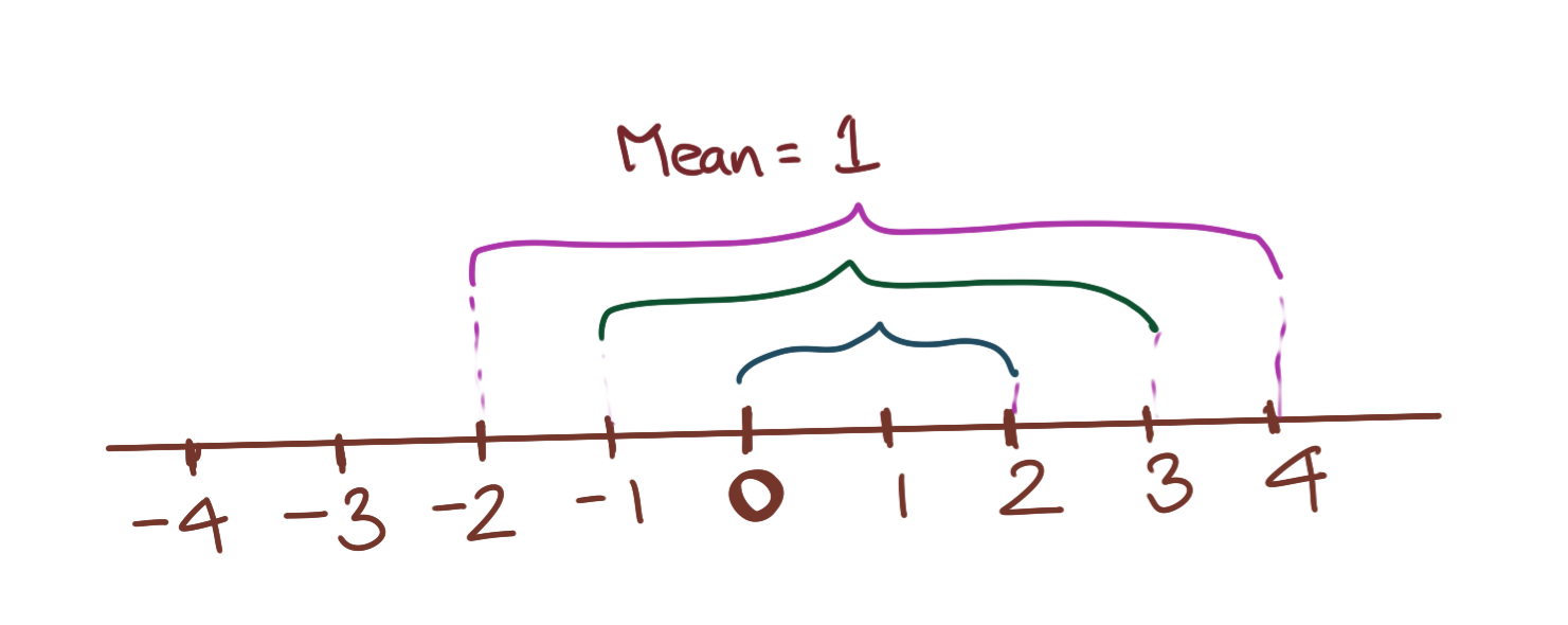
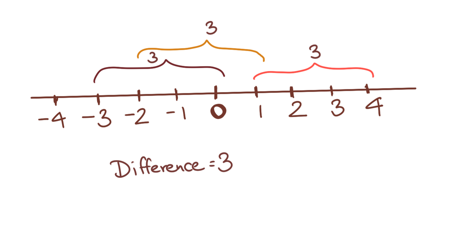
Let’s take a set of tuples. Each tuple contains two numbers, \(\mathbf{X=\{(1,3), (2,4), (7, 9)\}}\). If we’re asked to find the difference of each of these pairs of numbers, the answer is 2 in all cases. Note that the position of the mean keeps changing, as long as each pair of numbers moves in the smae direction at the same rate, i.e., (2,4) is the result of both ends of (1,3) moving by 1; the same idea applies to the other tuples. Thus, the mean in any of the above cases can always be written as \(b\), and each tuple of number can be written as \((b-k, b+k)\), where k is a constant. Then the difference is always \((b+k)-(b-k)=\mathbf{2k}\) in all cases.

This formulation will come in handy when we are expressing hyperplane intercepts later on, and exploring the possibilities of different hyperplane solutions for SVMs.

Equation of an Affine Hyperplane

The equation of a line in two dimensions passing through the origin, can always be written as:

\[ax+by=0\]

The equation of a line parallel to the above, but not passing through the origin, can be written as:

\[ax+by=c\]

\(ax+by=0\) is a linear subspace of \({\mathbb{R}}^2\) (see Subspace Intuitions). It is also, by definition, a hyperplane in \({\mathbb{R}}^2\).

\(ax+by=c\) is an affine subspace of \({\mathbb{R}}^2\). The simplistic definition of an affine subspace is a vector subspace which does not necessarily pass through the origin. There is a lot more subtlety involved where affine geometry is involved, but for the moment, the intuitive high-school equation of a general equation of a line in two dimensions will suffice. Extending this to a higher dimension \(N\), the equation of an affine hyperplane in \({\mathbb{R}}^N\) is:

\[\mathbf{w_1x_1+w_2x_2+...+w_{N-1}x_{N-1}=b}\]

The important thing to remember is that the dimensionality of a hyperplane is always one less than the dimensionality of the ambient space it inhabits; that’s why the indices in the above equation go up to \(N-1\).

Why is this the general form of the equation?
We can recover this general form with some simple matrix algebra. Let us assume that the hyperplane passing through the origin is represented by its normal \(N\). Then, since every point \(x\) on the hyoerplane is perpendicular to \(N\), we can write:

\[N^Tx=0\]

Let us now assume that this hyperplane has been displaced by an arbitrary vector \(u\); thus every point \(x\) has been displaced by a vector \(u\). To re-express the perpendicularity relationship, we must invert this displacement to bring the displaced hyperplane back to the origin, that is:

\[N^T(x-u)=0 \\ \Rightarrow N^Tx=N^Tu \\ \Rightarrow \mathbf{N^Tx=c} \\\]

The situation is shown below. Any \(x\) in the affine hyperplane is not perpendicular to the normal vector \(\vec{N}\). Only by translating it back to the original hyperplane (the linear subspace) can the perpendicularity relationship hold.

where \(c=N^Tu\), a constant, and the components of \(N\) are the weights \(w_1\), \(w_2\), etc.

An interesting result to note is when a hyperplane is displaced along its normal. Let us assume that \(c=tN\), where \(t\) is some arbitrary scalar. Then, substituting this into the relationship we derived, we get:

\[N^Tx=tN^TN \\ \Rightarrow N^Tx=t{\|N\|}^2 \\\]

Perpendicular Distance between two Parallel Affine Hyperplanes

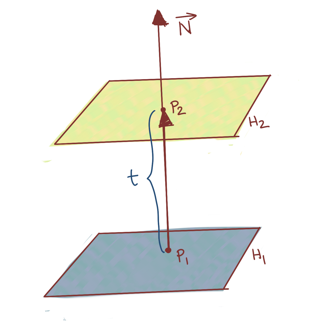
Next, we derive the perpendicular distance between two affine hyperplanes. Given two hyperplanes of the form:

\(N^Tx=c_1 ....(H_1)\)
\(N^Tx=c_2 ....(H_2)\)

we’d like to know the perpendicular distance between them. Note that they have the same normal because they are parallel, merely displaced from each other (and in this case, not passing through the origin, assuming \(c_1, c_2 \neq 0\)).

Assume a point \(P_1\) on \(H_1\), and a corresponding point \(P2\) on \(H_2\). Further, assume that the vector connecting these two points is the perpendicular

\[N^TP_1=c_1 \\ N^TP_2=c_2 \\ P_2=P_1+tN \\ \Rightarrow P_2-P_1=tN\]

The situation is show below:

Subtracting:

\[N^T(P_2-P_1)=c_2-c_1 \\ \Rightarrow N^T.tN=c_2-c_1 \\ \Rightarrow tN^TN=c_2-c_1 \\ \Rightarrow t{\|N\|}^2=c_2-c_1 \\ \Rightarrow \mathbf{t=\frac{c_2-c_1}{\|N\|^2}}\]

This recovers the scaling factor \(t\); we still need to multiply it with the magnitude of \(\vec{N}\) to give us the actual perpendicular distance between \(H_1\) and \(H_2\). Thus, the distance is:

\[d_perp(H_1,H_2)=t\|N\| \\ \Rightarrow d_perp(H_1,H_2)=\frac{c_2-c_1}{\|N\|^2}\|N\| \\ \Rightarrow \mathbf{d_{perp}(H_1,H_2)=\frac{c_2-c_1}{\|N\|}}\]

Let us perform a simple substitution where b is the mean of \(c_1\) and \(c_2\), i.e.,

\[b=\frac{c_1+c_2}{2}\]

and k is the distance from b to \(c_1\) and \(c_2\). Thus, we may write:

\[c_1=b-k \\ c_2=b+k\]

Consequently, the perpendicular distance between two affine hyperplanes can be rewritten as:

\[d_{perp}(H_1,H_2)=\frac{b+k-(b-k)}{\|N\|} \\ \Rightarrow \mathbf{d_{perp}(H_1,H_2)=\frac{2k}{\|N\|}}\]

Here’s the next question: what is the equation of the affine hyperplane halfway between \(H_1\) and \(H_2\). It is very tempting to assume that it is \(N^Tx=b\), but let us validate this intuition. The figure below shows the situation.

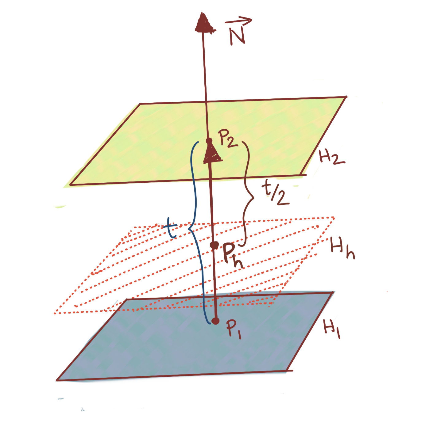
The scaling factor for this halfway hyperplane is obviously \(t/2=\frac{c_2-c_1}{2{\|N\|}^2}\). We use the same procedure we did when calculating the distance between \(H_1\) and \(H_2\), except this time we seek the intercept factor, and know the scaling factor already. Thus, if we write, for \(H_1\) and the halfway hyperplane \(H_h\):

\[N^TP_1=c_1 \\ N^TP_H=\beta \\ P_H-P_1=\frac{t}{2}N\]

Subtracting, we get:

\[N^T(P_H-P_1)=\beta -c_1 \\ \Rightarrow N^TN\frac{t}{2}=\beta -c_1 \\ \Rightarrow {\|N\|}^2\frac{c_2-c_1}{2{\|N\|}^2}=\beta -c_1 \\ \Rightarrow \frac{c_2-c_1}{2}=\beta -c_1 \\ \Rightarrow \mathbf{\beta=\frac{c_1+c_2}{2}=b}\]

This indeed corresponds with our intuition that an affine hyperplane midway between two parallel affine hyperplanes will have its intercept as the mean of those on either side of it.

Aside: Alternative Equivalent Solution

You can derive the same result, by assuming that you go along \(t/2\) times along vector \(\vec{N}\) starting from \(P_1\). That is:

\[P_H=P_1+\frac{t}{2}N\]

First, we multiply throughout by \(N^T\) to get:

\[N^TP_H=N^TP_1+\frac{t}{2}N^TN \\ \Rightarrow N^TP_H=N^TP_1+\frac{t}{2}{\|N\|}^2\]

Remembering that \(\mathbf{t=\frac{c_2-c_1}{\|N\|^2}}\) and \(N^TP_1=c_1\), we can write:

\[N^TP_H=c_1+\frac{c_2-c_1}{2{\|N\|}^2}{\|N\|}^2 \\ \Rightarrow N^TP_H=c_1+\frac{c_2-c_1}{2} \\ \Rightarrow \mathbf{N^TP_H=\frac{c_1+c_2}{2}}\]

which is the same result we’ve proved above.

Framing the SVM Optimisation Problem

We now have all the background we need to state the general problem Support Vector Machines are attempting to solve.

Separating Hyperplane

The primary purpose of SVMs is classification of training data. To put it very simply, we desire to find a affine hyperplane which can separate our data into two classes such that points in one class lie above the hyperplane, while all points in the other class, lie below the hyperplane.

The diagram below illustrates the concept.

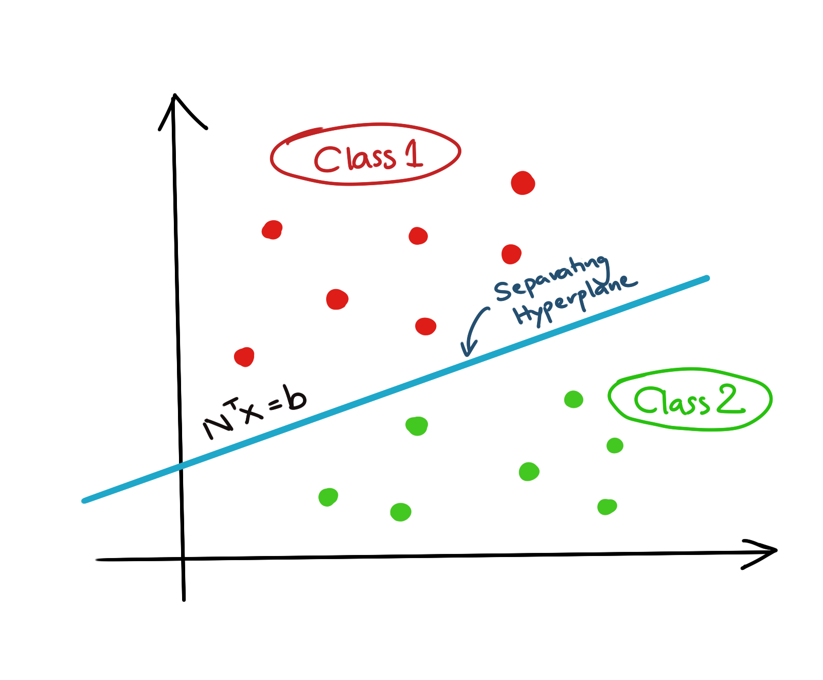
Let us state the first, and most important, assumption which accompanies this investigation, namely, that the data in the two classes, should be linearly separable. This implies that it should be possible to find a hyperplane, any hyperplane, in the first place which can separate the two classes of data neatly above and below the hyperplane.

Note: We will relax this assumption later, but for the moment, let us proceed with the simple case.

The second condition we impose on our solution will become clearer from the discussion below. If you look at the picture above, you’ll see that there is a lot of flexibility in terms of what this hyperplane can look like in terms of its parameters. In fact, in the example above, and very generally, there are an infinite number of hyperplanes which can partition the data into two classes perfectly, i.e., an infinite number of combinations of weights in the equation of the affine hyperplane. Here is an illustration of some example possibilities.

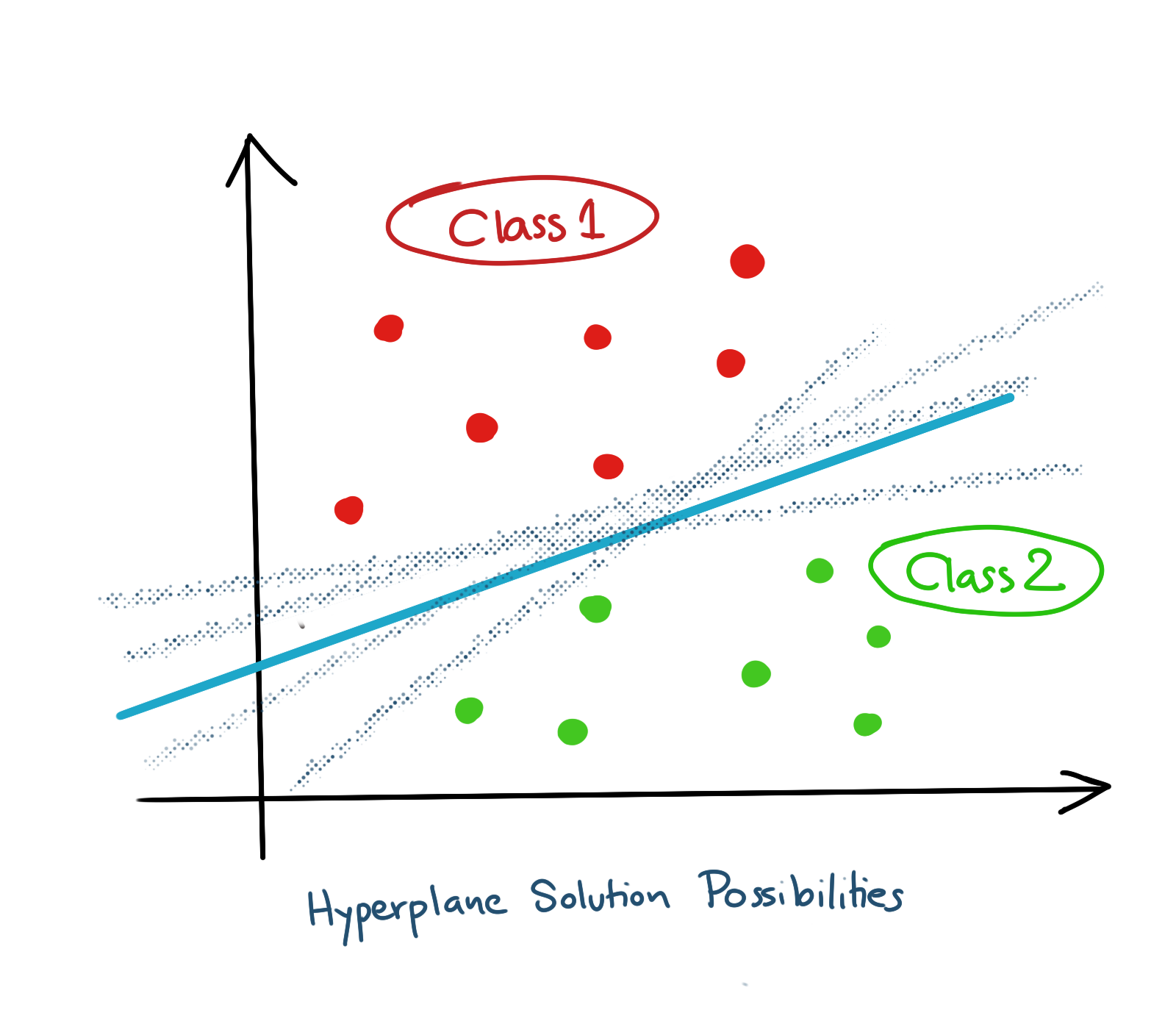
More data may constrain the space of solutions some more, but it will still be infinite in the most general case, assuming that the data is linearly separable. What combination should we choose?

This is where we’d like to impose some mathematical constraints on the solution to drive us toward a satisfactory solution. The most important one we have already stated, which is that all data points belonging to one class should fall on one side of the hyperplane. The second one is the one which gives Support Vector Machines their name. We’d like to maximise the Support Margin. What is a support margin? Let’s look at the diagram with a separating hyperplane once again.

Supporting Hyperplanes

If we take two points, one from each class, such that they are the closest to each other (there can be more than one of each type, but this argument extends to that as well), and draw two parallel hyperplanes through them (making sure that the points still say linearly separable), we will have drawn something like the dotted lines in the figure below.

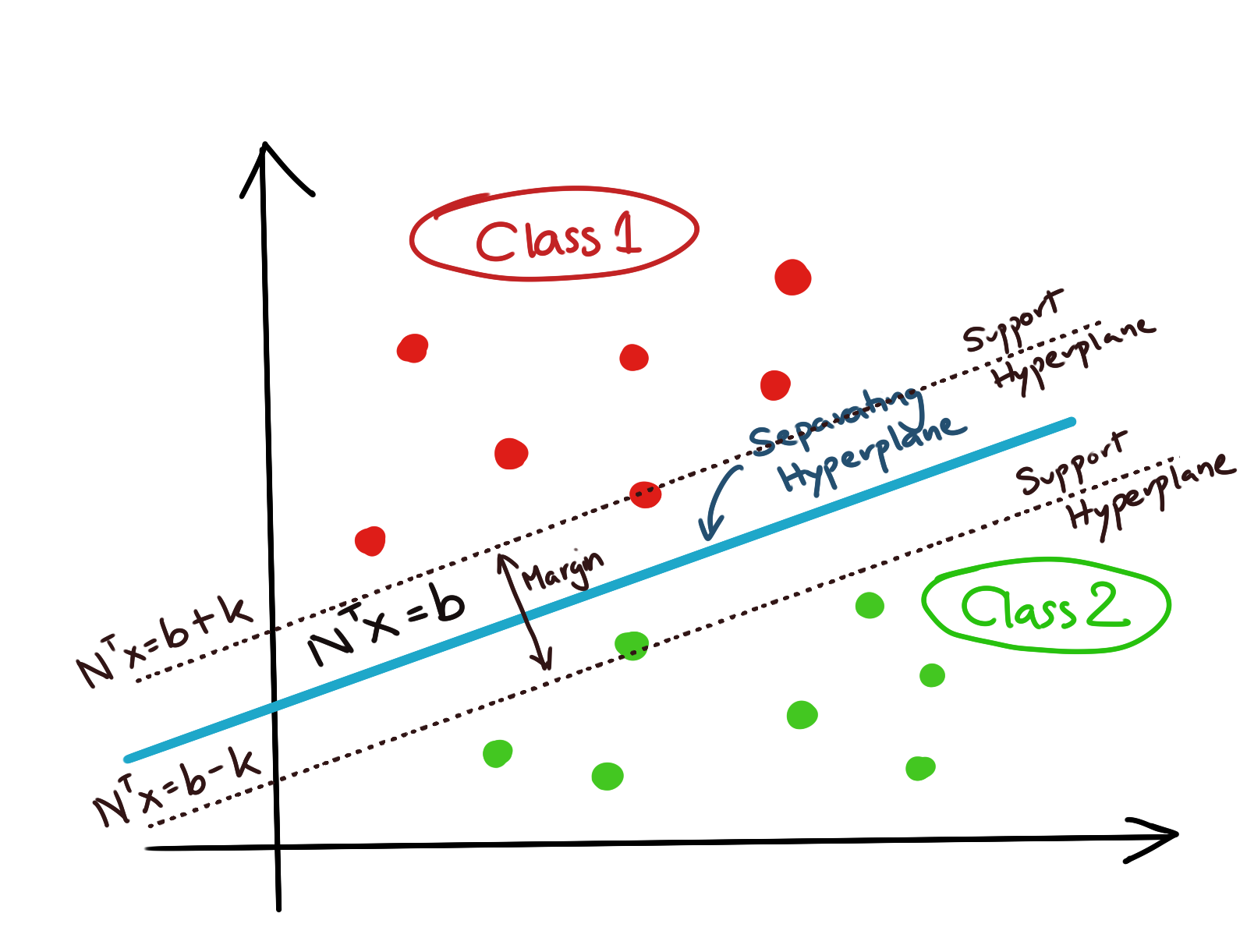
These hyperplanes that we’ve drawn are not the actual separating hyperplane, but they ‘bracket’ the actual hyperplane which will be used to classify our data. Thus, they are called the supporting hyperplanes of the SVM. The perpendicular distance between these supporting hyperplanes is the support margin of the Support Vector Machine. The actual separating hyperplane lies midway between these supporting hyperplanes.

Now, at face value, it might seem that we haven’t really improved our problem definition by a lot. After all, it is definitely possible to draw an infinite number of sets of supporting hyperplanes (and consequently, an infinite number of separating hyperplanes). The diagram below shows two possibilities: \(H_1\), \(H_{1-}\), and \(H_{1+}\) form one separating hyperplane-supporting hyperplane set, and \(H_2\), \(H_{2-}\), and \(H_{2+}\) form another.

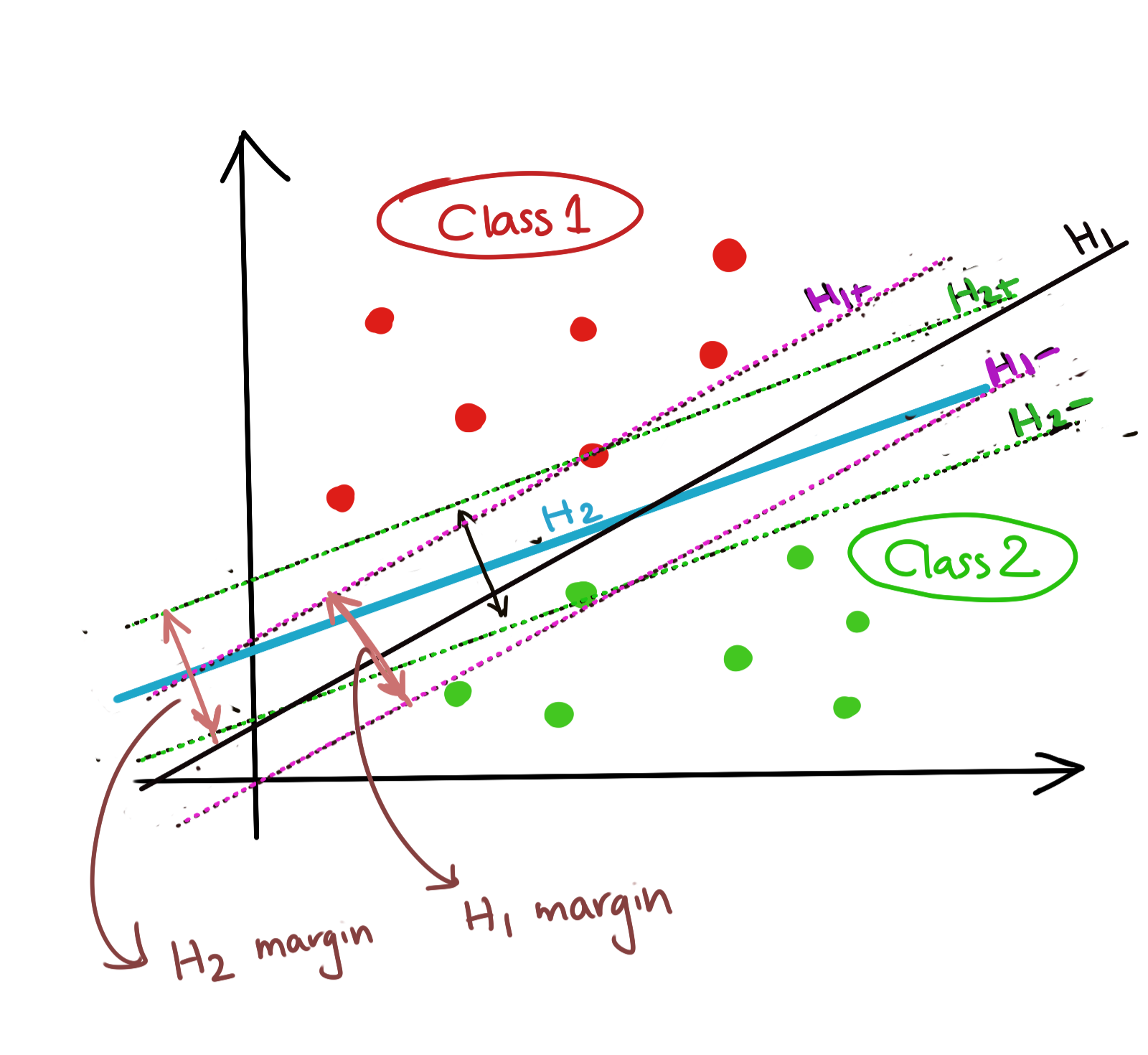
This is where we state the optimisation which will narrow down our solution space. We wish to find the set of supporting hyperplanes which maximises the support margin, subject to the constraints that all the data still stay linearly separable.

This immediately has an important implication: namely, that no data points may exist inside the margin of the SVM. This immediately puts more constraints on our solution because now the data points of class 1 in our example, need to not only fall above the separating hyperplane, they also need to be above or on the supporting hyperplane \(H_+\); the same argument holds for the other class.

Let us quantify all of these conditions mathematically. We seek a separating hyperplane of the form \(N^Tx=b\). We seek supporting hyperplanes of the form \(N^Tx=b+k\) and \(N^Tx=b-k\).

1. Linearly Separable Data

For a set of data \(x_i, i\in[1,N]\), if we assume that data is divided into two classes (-1,+1), we can write the constraint equations as:

\[\mathbf{ N^Tx_i\geq b+k, \forall x_i|y_i=+1 \\ N^Tx_i\leq b-k, \forall x_i|y_i=-1 }\]

2. Margin Maximisation

We have already derived the perpendicular distance between two affine hyperplanes of the form \(N^Tx=b+k\) and \(N^Tx=b-k\), which is \(\frac{2k}{\|N\|}\). We seek to obtain the following:

\[\mathbf{m_{max}=max \frac{2k}{\|N\|}}\]

This is an optimisation problem, which we will analyse in succeeding articles.

---