Quadratic Optimisation using Principal Component Analysis as Motivation: Part One

Avishek Sen Gupta on 19 April 2021

---

This series of articles presents the intuition behind the Quadratic Form of a Matrix, as well as its optimisation counterpart, Quadratic Optimisation, motivated by the example of Principal Components Analysis. PCA is presented here, not in its own right, but as an application of these two concepts. PCA proper will be presented in another article where we will discuss eigendecomposition, eigenvalues, and eigenvectors.

A succeeding post will explore the Quadratic Optimisation problem form, and the intuition behind the Lagrangian formulation.

One of the aims of this article is also to introduce PCA in a different context than eigenvectors, to show that there is more than one way to view a particular topic.

Parts of this should also serve as preliminaries for a couple of other topics:

• The Quadratic Form discussion will come in useful when talking of Gaussian Processes.
• The Quadratic Optimisation discussion will come in useful in deriving various results about Support Vector Machines.
• We will be better prepared for when I discuss Principal Components Analysis and Singular Value Decomposition, after this article.

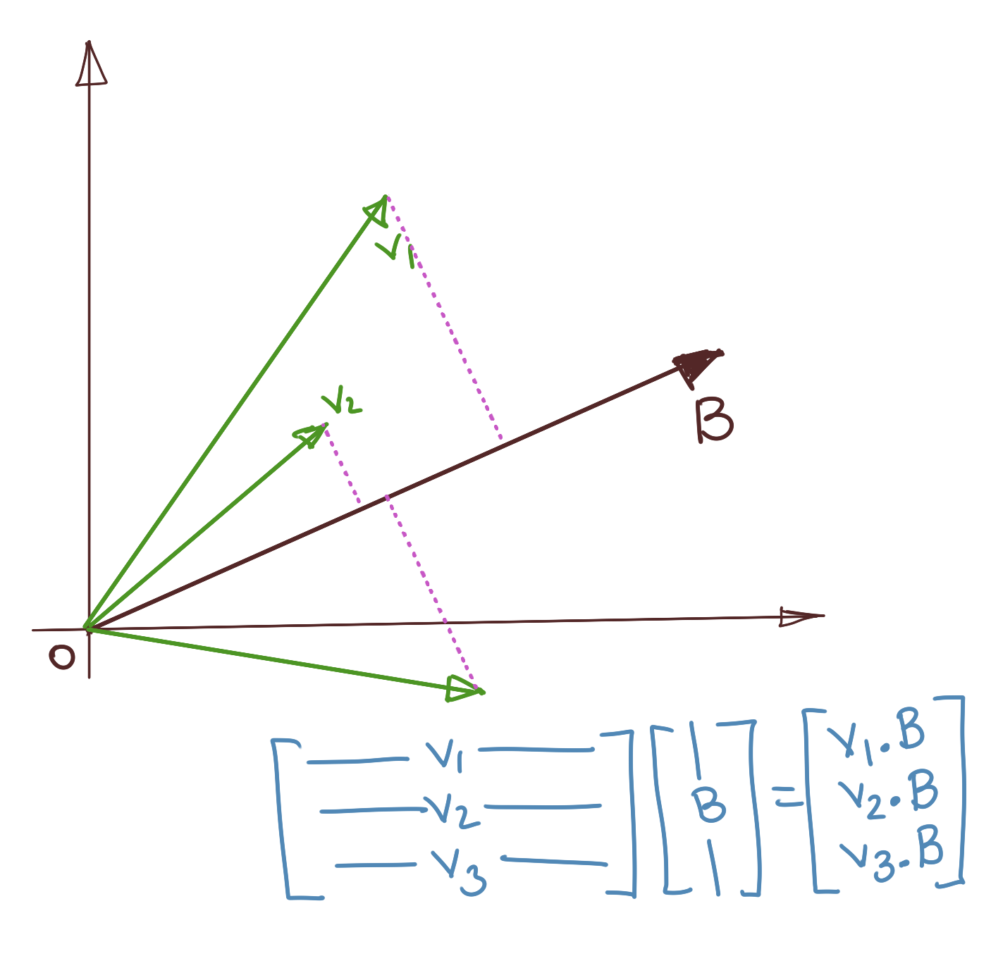
Preliminary: Computing the Dot Product of a set of vectors

This is not really a new concept, merely a reiteration of something that we will use as part of our optimisation-inspired derivation for Principal Components Analysis. We already know that the outer product of two matrices \(A\) and \(B\), let’s call it \(C\), has \(C_ik\) as the dot product of the \(i\)th row of \(A\) and the \(j\)th column of \(B\).

Specifically if we have a row vector \(A\) and a column vector \(B\), the normal vector outer product operation will yield the dot product \(A\cdot B\).

Generalising, instead of \(A\) being a single row vector, let it be a set of row vectors, i.e., a matrix \(O\times F\) (O=number of observations, F=number of variables, this will become relevant in a bit).

Then, the result of \(C=AB\) (where \(B\) is a \(F\times 1\) vector), will give us a \(O\times 1\) vector in which the \(i\)th entry will be the dot product of the \(i\)the row vector of \(A\) and the vector \(B\). More specifically, if \(B\) is a unit vector, the result is simply the projection of \(A\) on \(B\), since:

\(A\cdot B=\|A\|\|B\|cos\theta=\|A\|.1.cos \theta=\|A\|cos \theta\).

Geometrically, this gives us the projections of all the row vectors of \(A\) onto \(B\), assuming that \(B\) is a unit vector. This diagram explains the operation.

Preliminary: Variance

Variance essentially measures the degree of spread of a set of data around a mean value. This is also the same variance that is used to characterise a Gaussian Distribution. Given a set of data \(x_i\in\mathbb{R}, i\in[1,N]\) with a mean \(\mu\), variance is the average squared distance from the mean, i.e.,

\[\sigma^2=\frac{\sum_{i=1}^{N}{\|x_i-\mu\|}^2_2}{N}\]

where the subscript 2 indicates the L2 Norm or Euclidean Norm, which is nothing other than our basic distance formula. Let us simplify; we can always center the mean to the zero vector so that \(\mathbf{\mu=0}\), in which case, the above variance identity reduces to:

\[\sigma^2=\frac{\sum_{i=1}^{N}{\|x_i\|}^2}{N}\]

If \(x_i\) are entries in a \(N\times 1\) vector \(X\), the above can be re-expressed as:

\[\sigma^2=\frac{1}{N}\cdot X^TX\]

Principal Components Analysis as an Optimisation Problem

Let’s look at PCA and how we can express it, starting from one of its definitions. The intuition behind PCA will be explained more when we get to eigendecomposition; for the moment, we restrict ourselves to a more mechanical interpretation of PCA.

1. The Objective

From the Wikipedia definition of PCA:

The first principal component can equivalently be defined as a direction that maximizes the variance of the projected data. The \(i\)th principal component can be taken as a direction orthogonal to the first \(i-1\)th principal components that maximizes the variance of the projected data.

Alright, there’s a lot to unpack here, but I want to simplify and say very informally that PCA involves finding vectors which maximise the variance of a data set, when those vectors are used as basis vectors.

Consider a matrix \(X\), with one observation (data point) per row, each column representing a particular feature of this observation. Let there be \(O\) observations and \(F\) features. Thus, \(X\) is a \(O\times F\) matrix.

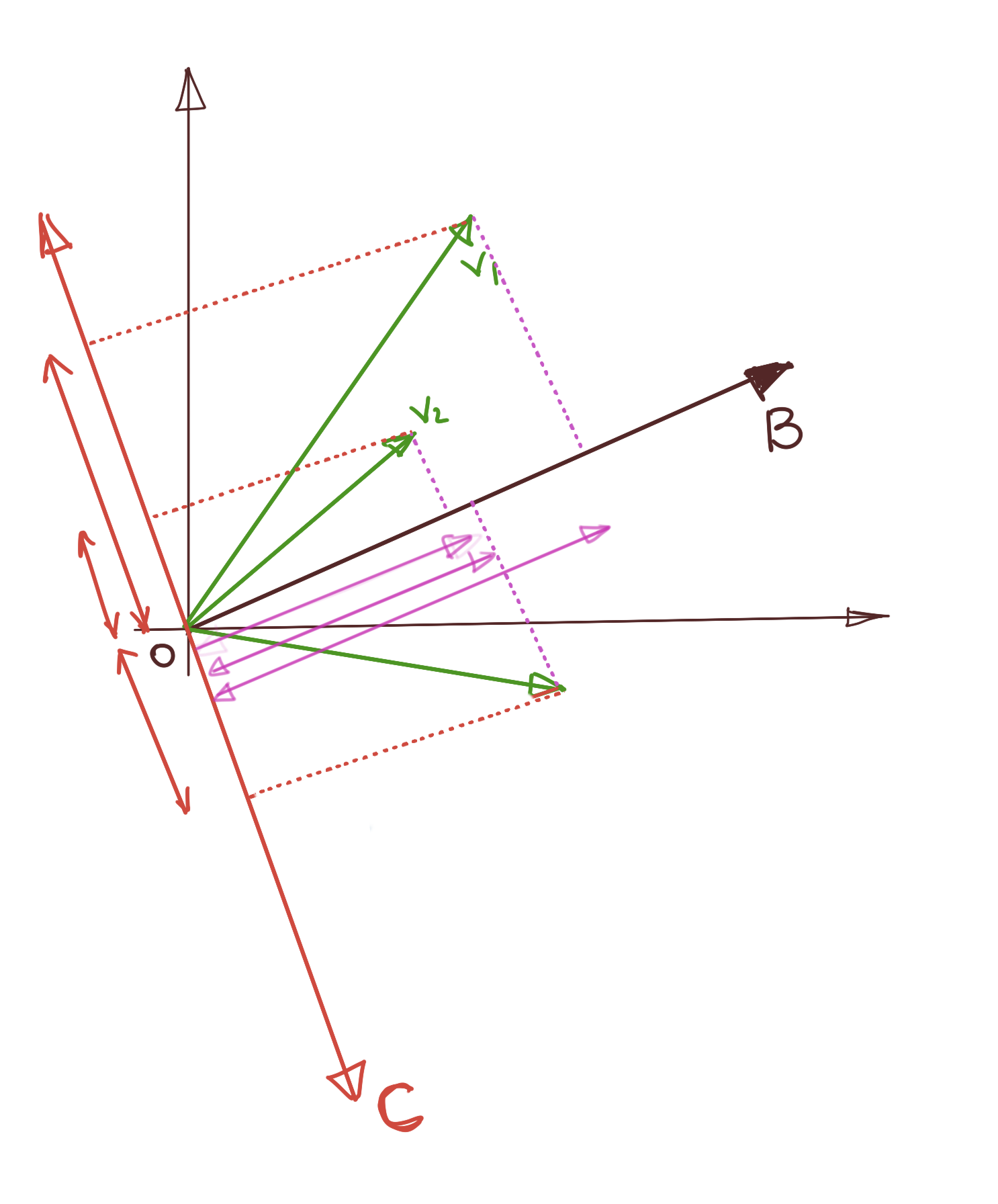
We’d like to project these data onto a vector such that the variance of these projected points onto that vector is maximised. There might be multiple vectors like this, but for the moment, let’s stick with finding one of them.

This picture explains the idea. As you can see, we can pick any random vector (\(B\) and \(C\) in the picture), and project our data onto it. These projections are scaled versions of this vector. We’d like the spread of these projections to be as dispersed as possible. For example, choosing \(C\) as a reference vector doesn’t seem to provide much spread (variance) for the data point \(V_2\), whereas choosing \(B\) as our reference vector provides a much larger variance to \(V_2\).

2. Variance of Projections

Let \(X\) be a set of row vectors, each representing, say, a data point from our data set. \(F\) is a candidate Principal Component vector.

\(X\) is a \(O\times F\) matrix, \(V\) is a \(F\times 1\) vector, so the projection is a \(O\times 1\) vector, the \(i\)th entry corresponding to the projection (a single number) of the \(i\)th row vector in \(X\) onto \(V\).

\[W=XV\]

Variance is thus:

\[W^TW={(XV)}^TXV \\ \Rightarrow W^TW=V^TX^TXV \Rightarrow W^TW=V^T\Sigma V\]

We ignore the division by \(N\), because that is merely a scaling factor which will not really affect framing our optimisation problem. It is important to note that \(\Sigma\) is a symmetric matrix, because it is a product of a matrix and its transpose.

2.1 Aside: The product of a matrix and its transpose is symmetric - Proof

\(A\) is an \(M\times N\) matrix. Consider the product of \(A^T\) and \(A\):

\[C_{ik}=\sum_{j=1}^N A^T_{ij}A_{jk} \\ C_{ki}=\sum_{j=1}^N A^T_{kj}A_{ji}\]

By definition of transpose, we have: \(A^T_{ij}=A_{ji} \\ A^T_{kj}=A_{jk}\)

Substituting the above in the first identity above, we get:

\[C_{ik}=\sum_{j=1}^N A_{ji}A^T_{kj} \\ \Rightarrow C_{ik}=\sum_{j=1}^N A^T_{kj}A_{ji}=C_{ki} \\\]

Thus, \(C\) is symmetric.

3. Maximise Variance

We thus need to find a vector \(V\) which maximises the expression \(V^TX^TXV\). We express this as:

Maximise \(V^T\Sigma V\)
Subject to: \(V^TV=1\)

The constraint \(V^TV=1\) is present because we’d like \(V\) to be a unit vector. Thus, we have formulated the definition of Principal Components Analysis, i.e., finding a set of vectors which maximise the variance of a data set when those vectors are used as the basis.

Of course, there is a lot to be said about eigendecomposition, but take particular note of the form of the cost function. Very generally, it is \(xQx^T\) or \(x^TQx\) (depending upon how you have structured your data). This form arises quite often in general optimisation problems, and obviously, is very important in Linear Algebra. This belongs to the class of optimisation called Quadratic Optimisation.

We will explore optimisation in a little bit, but let us focus on the Quadratic Form of a Matrix first.

Quadratic Form of a Matrix

The quadratic form of a matrix is always of the form \(\mathbf{x^TQx}\) where \(x\) is a column vector, and usually is the thing that varies. In quadratic optimisation problems, we usually attempt to determine \(x\) which optimises (maximises) the form \(x^TQx\), subject to one or more constraints.

Thus, it is instructive to study the shape of \(x^TQx\). Before looking at that, let us state some important assumptions about the shape of \(x\) and \(Q\).

• \(x\) is a \(N\times 1\) column vector, thus \(x^T\) is a \(1\times N\) row vector.
• \(Q\) is a square \(N\times N\) symmetric vector. We will examine in a second why this is not a limiting constraint at all.

Let’s take the two-dimensional case as an example, where:

\[x=\begin{bmatrix} x \\ y \end{bmatrix} \\ Q=\begin{bmatrix} a && b \\ b && c \\ \end{bmatrix}\]

Let us compute \(x^TQx\):

\[x^TQx= \begin{bmatrix} x && y \end{bmatrix} \begin{bmatrix} a && b \\ b && c \\ \end{bmatrix} \begin{bmatrix} x \\ y \end{bmatrix} \\ =\begin{bmatrix} x && y \end{bmatrix} \begin{bmatrix} ax+by \\ bx+cy \end{bmatrix} \\ =ax^2+2bxy+cy^2 \\ f(x,y)=\mathbf{ax^2+2bxy+cy^2}\]

This is the quadratic form of a \(2\times 2\) matrix. Note that the result is a scalar. Also, note how every term incorporates a product of exactly two variables. Thus, it is a homogenous polynomial. This degree (or the number of variables in a term) does not vary for higher dimensional vectors.

With that out of the way, it is time to look at the shape of this curve, so that we can build up our intuition of the Quadratic Program formulation. Of course, we cannot visualise dimensions higher than 3, so in the following discussion, all diagrams will incorporate two feature variables (\(x_1\) and \(x_2\)), and the third dimension is the value of the polynomial \(f(x_1,x_2)\).

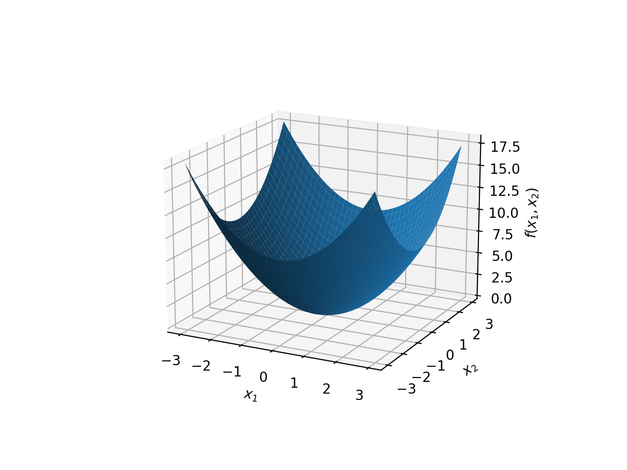
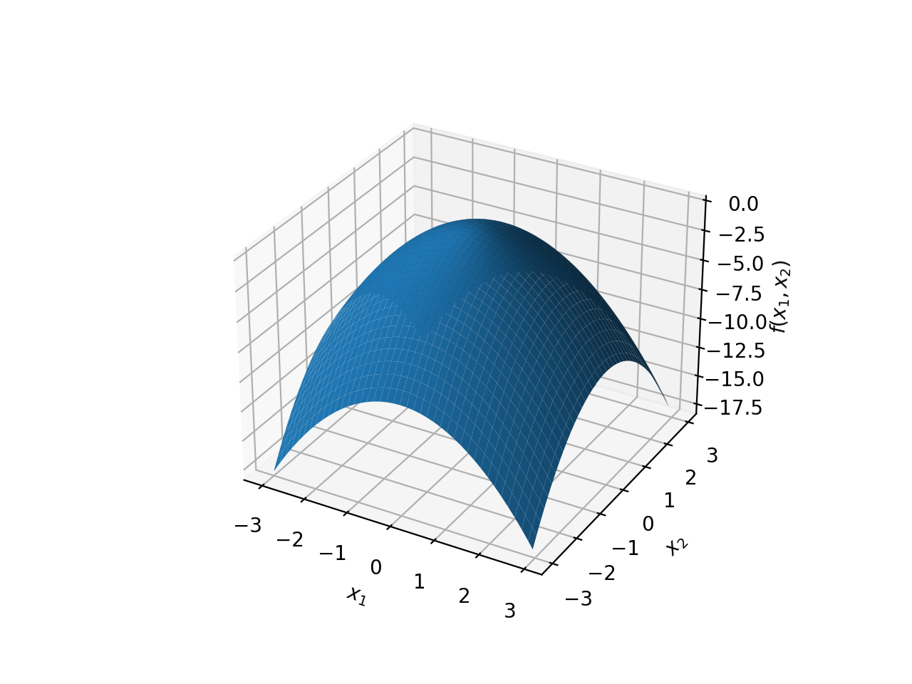
Here are some of the different surfaces, corresponding to what kind of coefficients exist in the quadratic polynomial.

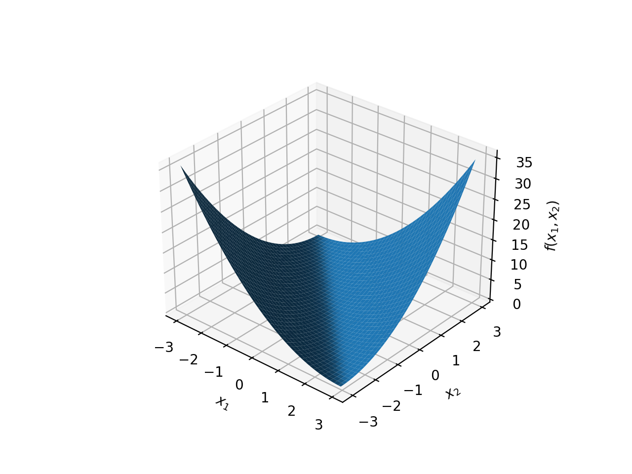
\(f(x)={x_1}^2+{x_2}^2\)

---

\(f(x)=-{x_1}^2-{x_2}^2\)

---

\(f(x)={x_1}^2-{x_2}^2\)

---

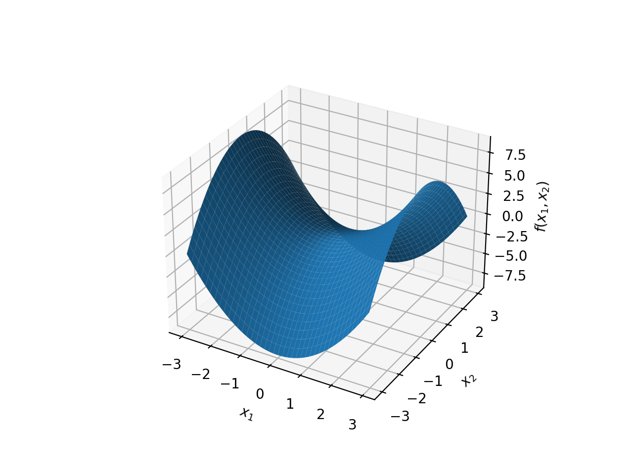
\(f(x)={x_1}^2-{x_2}^2-2{x_1}{x_2}\)

---

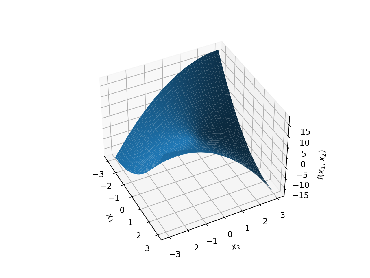
\(f(x)={x_1}^2+{x_2}^2+2{x_1}{x_2}\)

---

The above graphs show only a part of the quadratic surfaces, because they extend infinitely in all directions.

We will have a lot more to talk about quadratic surfaces when we tackle eigendecomposition proper, but for the moment, understand that Quadratic Optimisation problems involve searching for a combination of variables \((x_1, x_2,...,x_N)\) which find the global maximum on these surfaces, subject to particular constraints on \(x_i\).

That last phrase about constraints is particularly important. This is because all these quadratic surfaces extend infinitely in all directions, and you can make your variables as large as you want, if there are no constraints. For example, in the figure where \(f(x)={x_1}^2+{x_2}^2x\), if we are asked to maximise \(f(x)\), we can easily see that the function rises high towards infinity as \((x_1, x_2)\) move towards infinity. Thus, it is nonsensical (in many cases) to ask for optimisation if constraints are not present.

However, it is important to note that some problems may have a constraint on them, but that constraint might not be activated while searching for a solution. We will discuss these situations in a succeeding post when we introduce the intuition behind Lagrangian Optimisation, because combining all these conditions, gives us an important result in Quadratic Optimisation, the Karush-Kuhn-Tucker Conditions (KKT in short).

Invariability of Quadratic Polynomial under Symmetric Matrix Reformulation

Quadratic Optimisation problems involve matrices because they are a compact way of representing the problem. However, the actual optimisation revolves around the quadratic polynomial itself. This implies that we can modify our matrix to be anything as long as the resulting quadratic polynomial is the same.

I noted earlier than one important assumption in Quadratic Optimisation is that the matrix \(Q\) in the expression \(x^TQx\) is a symmetric matrix. What if we are given a matrix \(P\) which is not symmetric?

We seek to reformulate this matrix \(P\) such that it ends up being symmetric without affecting the resultant polynomial. To see how we can do this, it is instructive to look at the contribution of the matrix P to any of the cross terms of the polynomial.

Very generally, if we have a vector of N variables \(x_1, x_2,...,x_N\), the contribution of the matrix \(P\) to the coefficient of the cross term \(x_ix_j\) is the sum \(P_{ij}+P_{ji}\). You can see this when we computed the quadratic form of \(P=\begin{bmatrix} a && b \\ b && c \\ \end{bmatrix}\)

The polynomial came out as \(x^2+y^2+2bxy\). The entries \((1,2)\) and \((2,1)\) contributed to give \(2b\) as the coefficient of the \(xy\) term. You can verify this yourself for higher dimensional vectors.

Thus, if we take \(\mathbf{Q=\frac{1}{2}(P^T+P)}\), we get:

\[Q_{ij}=\frac{1}{2}(P_{ij}+P_{ji}) \\ Q_{ji}=\frac{1}{2}(P_{ji}+P_{ij})=Q_{ij}\]

Thus, \(Q\) is symmetric. Now,if we use \(Q\) to compute the polynomial, we get for the coefficient of the \(x_ix_j\) cross-term:

\[Q_{ij}+Q_{ji}=\frac{1}{2}(P_{ij}+P_{ji})+\frac{1}{2}(P_{ji}+P_{ij}) \\ \Rightarrow \mathbf{Q_{ij}+Q_{ji}=P_{ij}+P_{ji}}\]

Thus, computing \(Q\)’s quadratic form is the same as computing \(P\)’s quadratic polynomial, plus we have \(Q\) as symmetric, which is what we set out to do.

The next part of this series of post will clarify some basic understanding of Vector Calculus, specifically around gradients, so as to making understanding the Lagrangian formulation easier.

---