Quadratic Optimisation: Mathematical Background

Avishek Sen Gupta on 8 May 2021

---

This article continues the original discussion on Quadratic Optimisation, where we considered Principal Components Analysis as a motivation. Originally, this article was going to begin delving into the Lagrangian Dual and the Karush-Kuhn-Tucker Theorem, but the requisite mathematical machinery to understand some of the concepts necessitated breaking the preliminary setup into its own separate article (which you’re now reading).

Affine Sets

Take any two vectors \(\vec{v_1}\) and \(\vec{v_2}\). All the vectors (or points, if you so prefer) along the line joining the tips of \(\vec{v_1}\) and \(\vec{v_2}\) obviously lie on a straight line. Thus, we can represent any vector along this line segment as:

\[\vec{v}=\vec{v_1}+\theta(\vec{v_1}-\vec{v_2}) \\ =\theta \vec{v_1}+(1-\theta)\vec{v_2}\]

We say that all these vectors (including \(\vec{v_1}\) and \(\vec{v_2}\)) form an affine set. More generally, a vector is a member of an affine set if it satisfies the following definition.

\[\vec{v}=\theta_{1} \vec{v_1}+\theta_{2} \vec{v_2}+...+\theta_{n} \vec{v_n} \\ \theta_1+\theta_2+...+\theta_n=1\]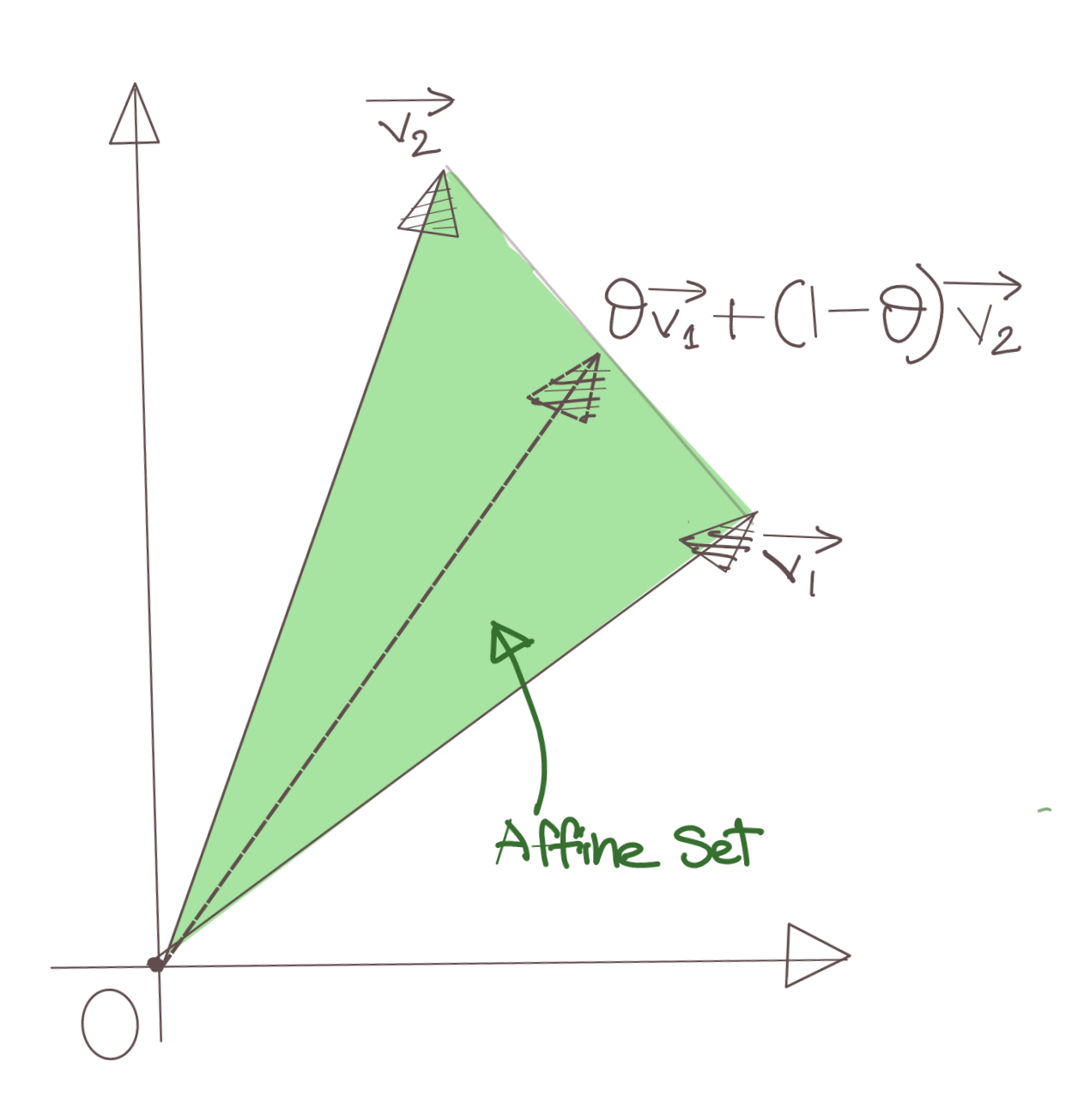

In words, a vector is an affine combination of \(n\) vectors if the coefficients of the linear combinations of those vectors sum to one.

Convex and Non-Convex Sets

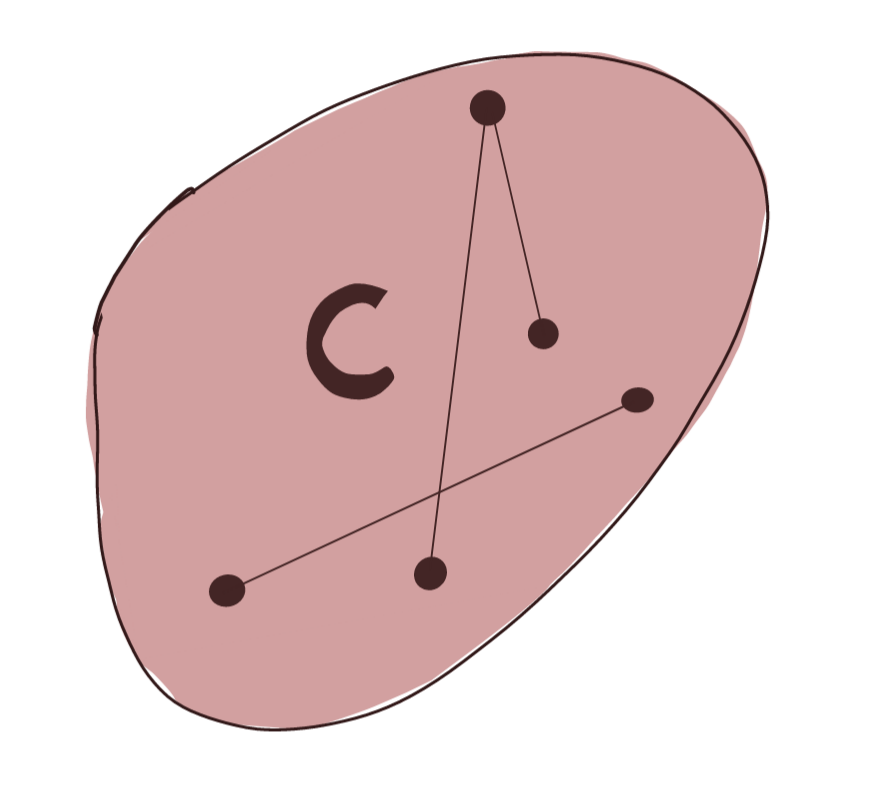
A set is said to be a convex set if for any two points belonging to the set, all their affine combinations also belong to the set. In simpler times, it means that a straight line between two points belonging to a convex set, lies completely inside the set.

Mathematically, the condition for convexity is the following:

\[\theta p_1+(1-\theta)p_2 \in C, \text{ if } p_1,p_2 \in C\]

The set shown below is a convex set.

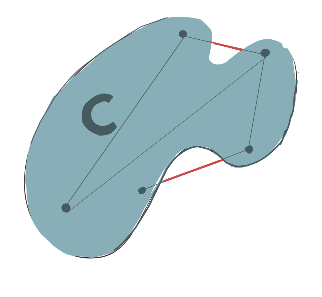
Any set that does not adhere to the above definition, is, by definition, a nonconvex set.

The set below is nonconvex. The red segments of the lines joining the points within the set lie outside the set, and thus violate the definition of convexity.

Convex and Concave Functions

The layman’s explanation of a convex function is that it is a bowl-shaped function. However, let us state this mathematically: we say a function is convex, if the graph of that function lies below every point on a line connecting any two points on that function.

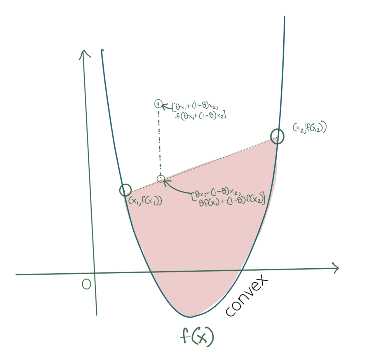
If \((x_1, f(x_1))\) and \((x_2, f(x_2))\) are two points on a function \(f(x)\), then \(f(x)\) is convex iff:

\[\mathbf{f(\theta x_1+(1-\theta x_2))\leq \theta f(x_1)+(1-\theta)f(x_2)}\]

Consider a point \(P\) on the line connecting \([x_1, f(x_1)]\) and \([x_2, f(x_2)]\), its coordinate on that line is \([\theta x_1+(1-\theta) x_2, \theta f(x_1)+(1-\theta) f(x_2)]\). The corresponding point on the graph is \([\theta x_1+(1-\theta) x_2, f([\theta x_1+(1-\theta) x_2)]\).

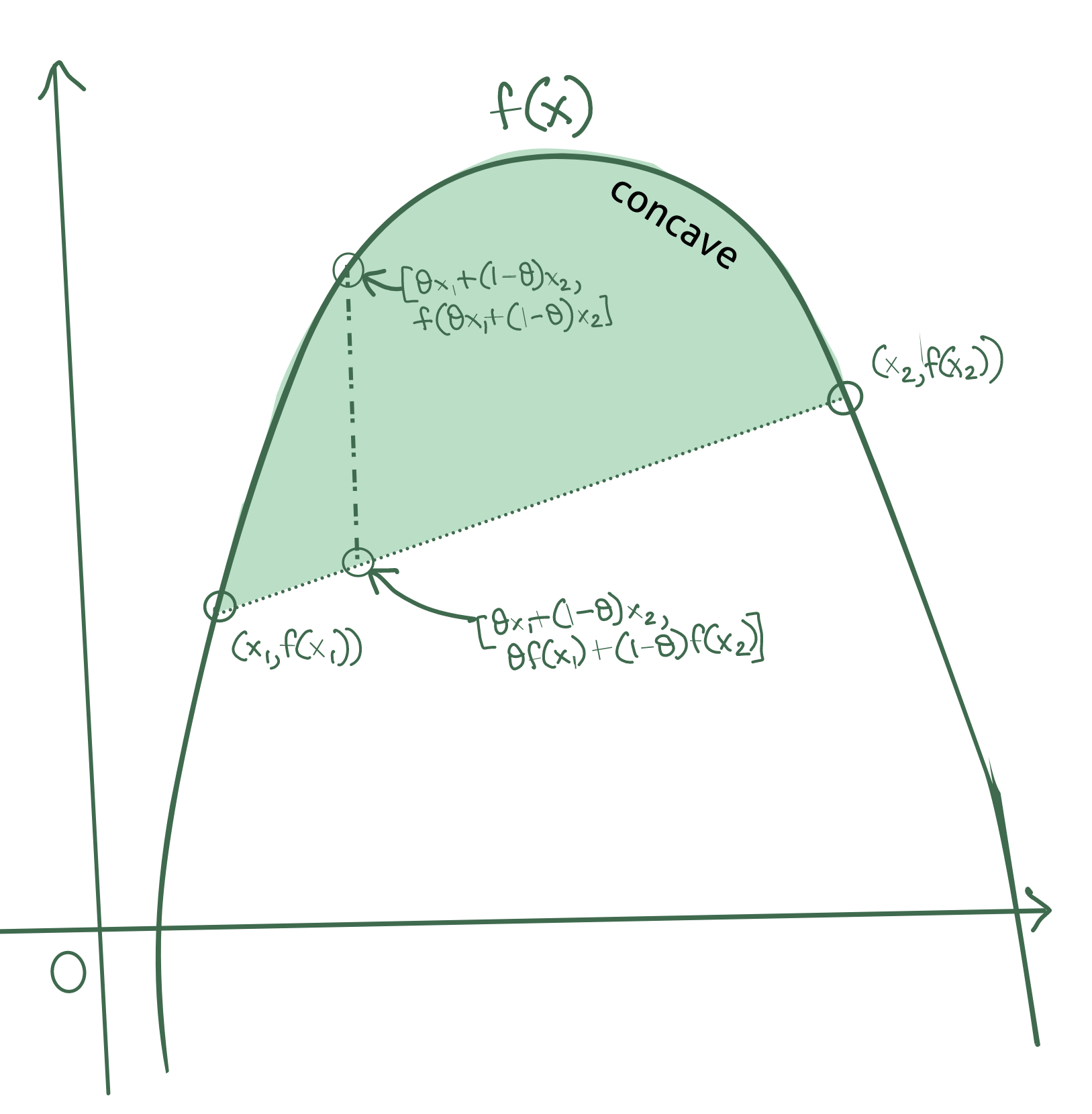The same condition, but inverted, can be applied to define a concave function. A function \(f(x)\) is concave iff:

\[\mathbf{f(\theta x_1+(1-\theta x_2))\geq \theta f(x_1)+(1-\theta)f(x_2)}\]

Affine Functions

An function \(f(x)\) is an affine function iff:

\[\mathbf{f(\theta x_1+(1-\theta) x_2)=f(\theta x_1)+f((1-\theta) x_2)}\]

Let’s take a simple function \(f(x)=Ax+C\) where \(x\) is a vector. \(A\) is a transformation matrix, and \(C\) is a constant vector. Then, for two vectors \(\vec{v_1}\) and \(\vec{v_2}\), we have:

\[f(\theta \vec{v_1}+(1-\theta) \vec{v_2})=A.[\theta \vec{v_1}+(1-\theta) \vec{v_2}]+C \\ =A\theta \vec{v_1}+A(1-\theta) \vec{v_2}+(\theta+1-\theta)C \\ =A\theta \vec{v_1}+A(1-\theta) \vec{v_2}+\theta C+(1-\theta)C \\ =[\theta A\vec{v_1}+\theta C]+[(1-\theta) A\vec{v_2}+(1-\theta)C]\\ =\theta[A\vec{v_1}+C]+(1-\theta)[A\vec{v_2}+C]\\ =\theta f(\vec{v_1})+(1-\theta) f(\vec{v_2})\]

Thus all mappings of the form \(\mathbf{f(x)=Ax+C}\) are affine functions.

We may draw another interesting conclusion: affine functions are both convex and concave. This is because affine functions satisfy the equality conditions for both convexity and concavity: an affine set on an affine function lies fully on the function itself.

Supporting Hyperplanes

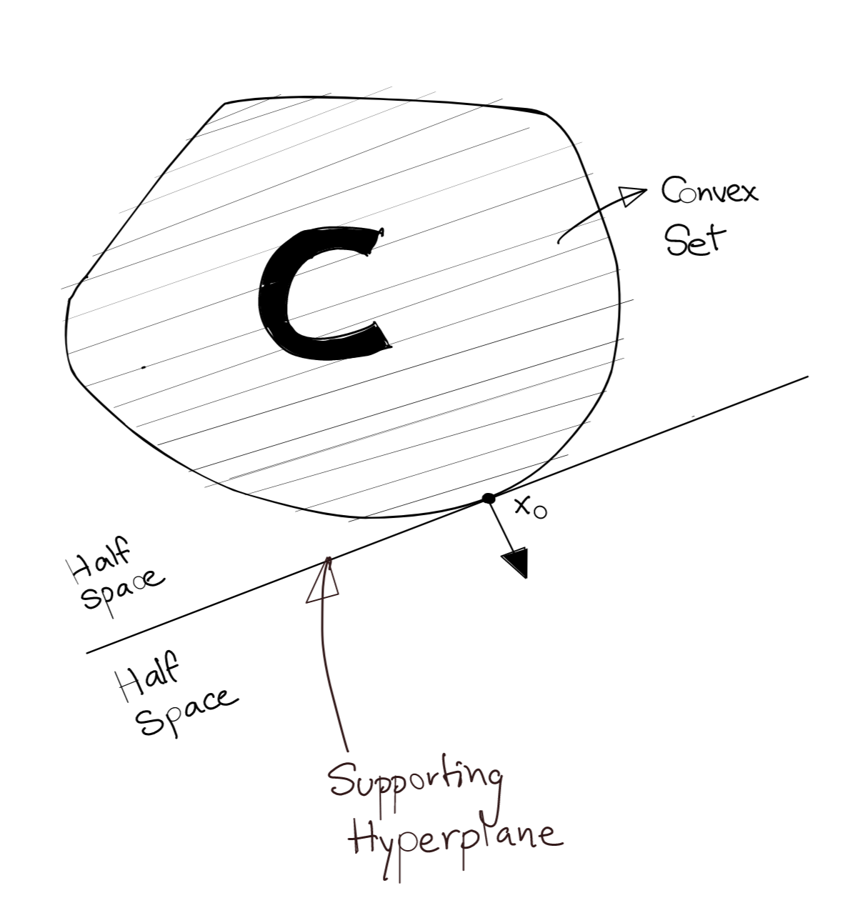
A supporting hyperplane for a set \(C\) is a hyperplane which has the following properties:

• The supporting hyperplane is guaranteed to contain at least one point which is also on the boundary of the set \(C\).
• The supporting hyperplane divides \(\mathbb{R}^n\) into two half-spaces such that set \(C\) is completely contained by one of these half-spaces.

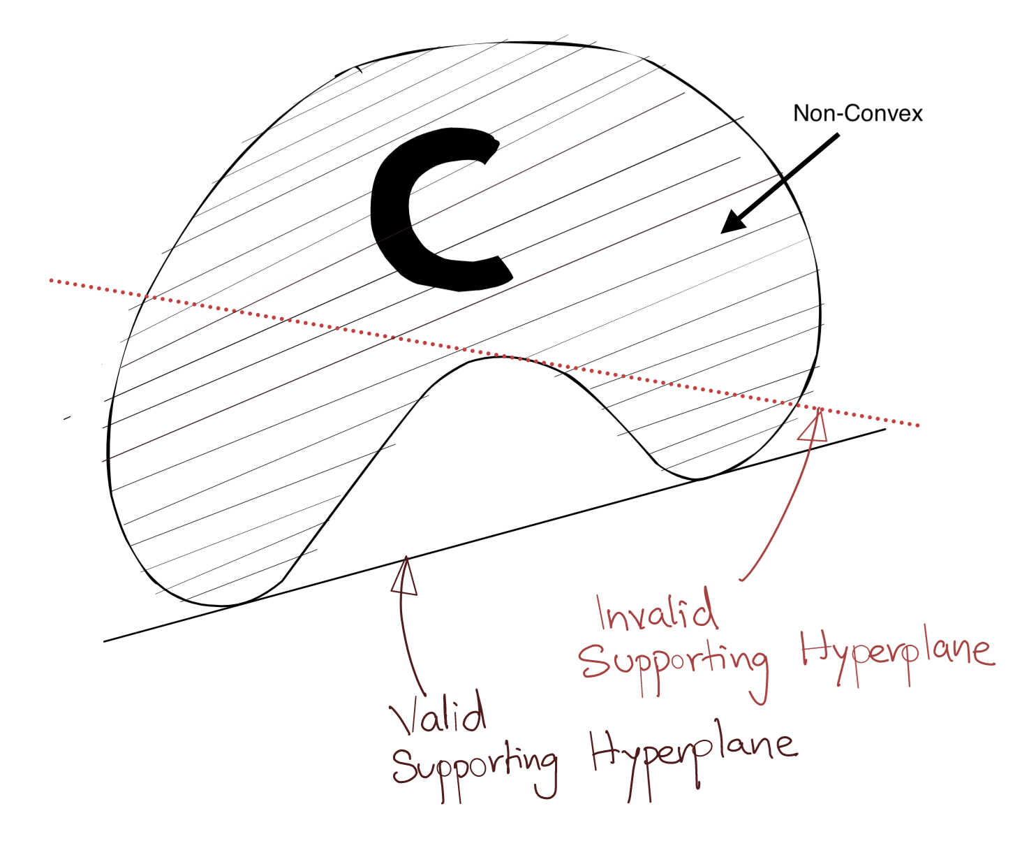
The definition of a convex set can also be explained by supporting hyperplanes. If there exists at least one supporting hyperplane for each point on the boundary of a set \(C\), \(C\) is convex.

The diagram below shows an example of a supporting hyperplane for a convex set.

The diagram below shows an example of an invalid supporting hyperplane (the dotted hyperplane). The dotted supporting hyperplane cannot exist because set \(C\) lies in both the half-spaces defined by this hyperplane.

Some Inequality Proofs

Result 1

If \(a\geq b\), and \(c\geq d\), then:

\[min(a,c)\geq min(b,d)\]

The proof goes like this, we can define the following inequalities in terms of the \(min\) function:

\[\begin{eqnarray} a \geq min(a,c) \label{eq:1} \\ c \geq min(a,c) \label{eq:2} \\ b \geq min(b,d) \label{eq:3} \\ d \geq min(b,d) \label{eq:4} \\ \end{eqnarray}\]

Then, the identities \(a \geq b\) and \(\eqref{eq:3}\) imply:

\[a \geq b \geq min(b,d)\]

Similarly, the identities \(c \geq d\) and \(\eqref{eq:4}\) imply that:

\[c \geq d \geq min(b,d)\]

Therefore, regardless of our choice from \(a\), \(c\) from the function \(min(a,c)\), the result will always be greater than \(min(b,d)\). Thus we write:

\[\begin{equation} \mathbf{min(a,c) \geq min(b,d)} \label{ineq:1}\end{equation}\]

Result 2

Here we prove that:

\[min(a+b, c+d) \geq min(a,c)+min(b,d)\]

Here we take a similar approach, noting that:

\[a \geq min(a,c) \\ c \geq min(a,c) \\ b \geq min(b,d) \\ d \geq min(b,d) \\\]

Therefore, if we compute \(a+b\) and \(c+d\), we can write:

\[a+b \geq min(a,c)+min(b,d) \\ c+d \geq min(a,c)+min(b,d)\]

Therefore, regardless of our choice from \(a+b\), \(c+d\) from the function \(min(a+b,c+d)\), the result will always be greater than \(min(a,c)+min(b,d)\). Thus we write:

\[\begin{equation}\mathbf{min(a+b, c+d) \geq min(a,c)+min(b,d)} \label{ineq:2} \end{equation}\]

Infimum and Supremum

The infimum of a function \(f(x)\) is defined as:

\[\mathbf{inf_x(f(x))=M | M<f(x) \forall x}\]

The infimum is defined for all functions even if the minimum does not exist for a function, and is equal to the mimimum if it does exist.

The supremum of a function \(f(x)\) is defined as:

\[\mathbf{sup_x(f(x))=M | M>f(x) \forall x}\]

The supremum is defined for all functions even if the maximum does not exist for a function, and is equal to the maximum if it does exist.

Pointwise Infimum and Pointwise Supremum

The pointwise infimum of two functions \(f_1(x)\) and \(f_2(x)\) is defined as thus:

\[pinf(f_1, f_2)=min\{f_1(x), f_2(x)\}\]

The pointwise supremum of two functions \(f_1(x)\) and \(f_2(x)\) is defined as thus:

\[psup(f_1, f_2)=max\{f_1(x), f_2(x)\}\]

We’ll prove an interesting result that will prove useful when exploring the shape of the Lagrangian of the objective function, namely that the pointwise infimum of any set of concave functions is a concave function.

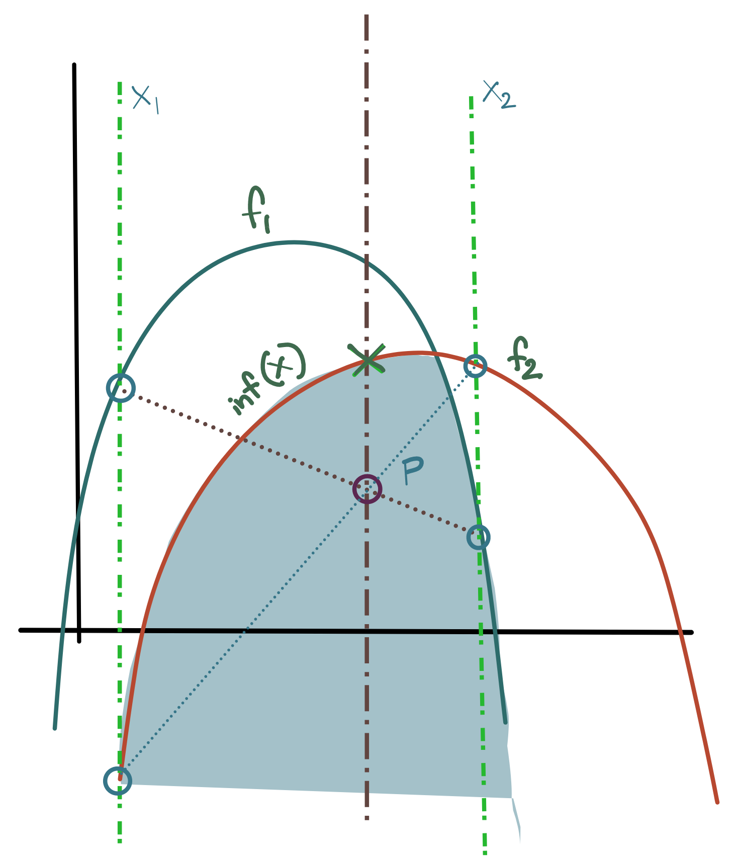
Let there be a chord \(C_1\) connecting (x_1, f_1(x_1)) and (x_2, f_1(x_2)) for a concave function \(f_1(x)\). Let there be a chord \(C_2\) connecting (x_1, f_2(x_1)) and (x_2, f_2(x_2)) for a concave function \(f_2(x)\).

Let us fix two arbitrary x-coordinates \(x_1\) and \(x_2\). Then, by the definition of a concave function (see above), we can write for \(f_1\) and \(f_2\):

\[f_1(\alpha x_1+\beta x_2)\geq \alpha f_1(x_1)+\beta f_1(x_2) \\ f_2(\alpha x_1+\beta x_2)\geq \alpha f_2(x_1)+\beta f_2(x_2)\]

where \(\alpha+\beta=1\). Let us define the pointwise infimum function as:

\[\mathbf{pinf(x)=min\{f_1(x), f_2(x)\}}\]

Then:

\[pinf(\alpha x_1+\beta x_2)=min\{ f_1(\alpha x_1+\beta x_2), f_2(\alpha x_1+\beta x_2)\} \\ \geq min\{ \alpha f_1(x_1)+\beta f_1(x_2), \alpha f_2(x_1)+\beta f_2(x_2)\} \hspace{4mm}\text{ (from }\eqref{ineq:1})\\ \geq \alpha.min\{f_1(x_1),f_2(x_1)\} + \beta.min\{f_1(x_2),f_2(x_2)\} \hspace{4mm}(\text{ from } \eqref{ineq:2})\\ = \mathbf{\alpha.pinf(x_1) + \beta.pinf(x_2)}\]

Thus, we can summarise:

\[\begin{equation} \mathbf{pinf(\alpha x_1+\beta x_2) \geq \alpha.pinf(x_1) + \beta.pinf(x_2)} \end{equation}\]

which is the form of an concave function, and thus we can conclude that \(pinf(x)\) is a concave function if all of its component functions are concave.

Since this is a general result for any two coordinates \(x_1,x_2:x_1,x_2 \neq 0\), we can conclude that the pointwise infimum of two concave functions is also a concave function. This can be extended to an arbitrary set of arbitrary concave functions.

Using very similar arguments, we can also prove that the pointwise supremum of an arbitrary set of convex functions is also a convex function.

The other straightforward conclusion is that the pointwise infimum of any set of affine functions is always concave, because affine functions are concave (they are also convex, but we cannot draw any general conclusions about the pointwise infimum of convex functions).

Note: The pointwise infimum and pointwise supremum have different definitions from the infimum and supremum, respectively.

The Max-Min Inequality

The Max-Min Inequality is a very general statement about the implications of ordering of maximisation/minimisation procedures along different axes of a function.

Fix a particular point \((x_0,y_0)\).

\[\text{ inf}_xf(x,y_0)\leq f(x_0,y_0)\leq \text{ sup}_yf(x_0,y)\]

This holds for any \((x_0,y_0)\), thus, we can simplify the notation, and omit the middle term to write:

\[\text{ inf}_xf(x,y)\leq \text{ sup}_yf(x,y) \\ g(x,y)\leq h(x,y) \text{ }\forall x,y\in\mathbf{R}\]

where \(g(x,y)=\text{ inf}_xf(x,y)\) and \(h(x,y)=\text{ sup}_yf(x,y)\). Note that at this point, \(g\) and \(h\) can be simple scalars or functions in their oown right; it depends upon the degree of the original function \(f(x,y)\).

In the general case, the infimum will define a function whose image will contain values which are all less than the smallest value in the image of the supremum function. We express this last statment as:

\[\sup_y g(x,y)\leq \inf_x h(x,y) \\ \Rightarrow \mathbf{\sup_y \text{ inf}_x f(x,y)\leq \inf_x \text{ sup}_y f(x,y)}\text{ }\forall x,y\in\mathbf{R}\]

This is the statement of the Max-Min Inequality.

The Minimax Theorem

The Minimax Theorem (first proof by John von Neumann) specifies conditions under which the Max-Min Inequality is an equality. This will prove useful in our discussion around solutions to the Lagrangian. Specifically, the theorem states that the

\[\mathbf{\sup_y \text{ inf}_x f(x,y)\leq \inf_x \text{ sup}_y f(x,y)} \text{ }\forall x,y\in\mathbf{R}\]

if:

• \(f(x,y)\) is convex in \(y\) (keeping \(x\) constant)
• \(f(x,y)\) is concave in \(x\) (keeping \(y\) constant)

The diagram below shows the graph of such a function.

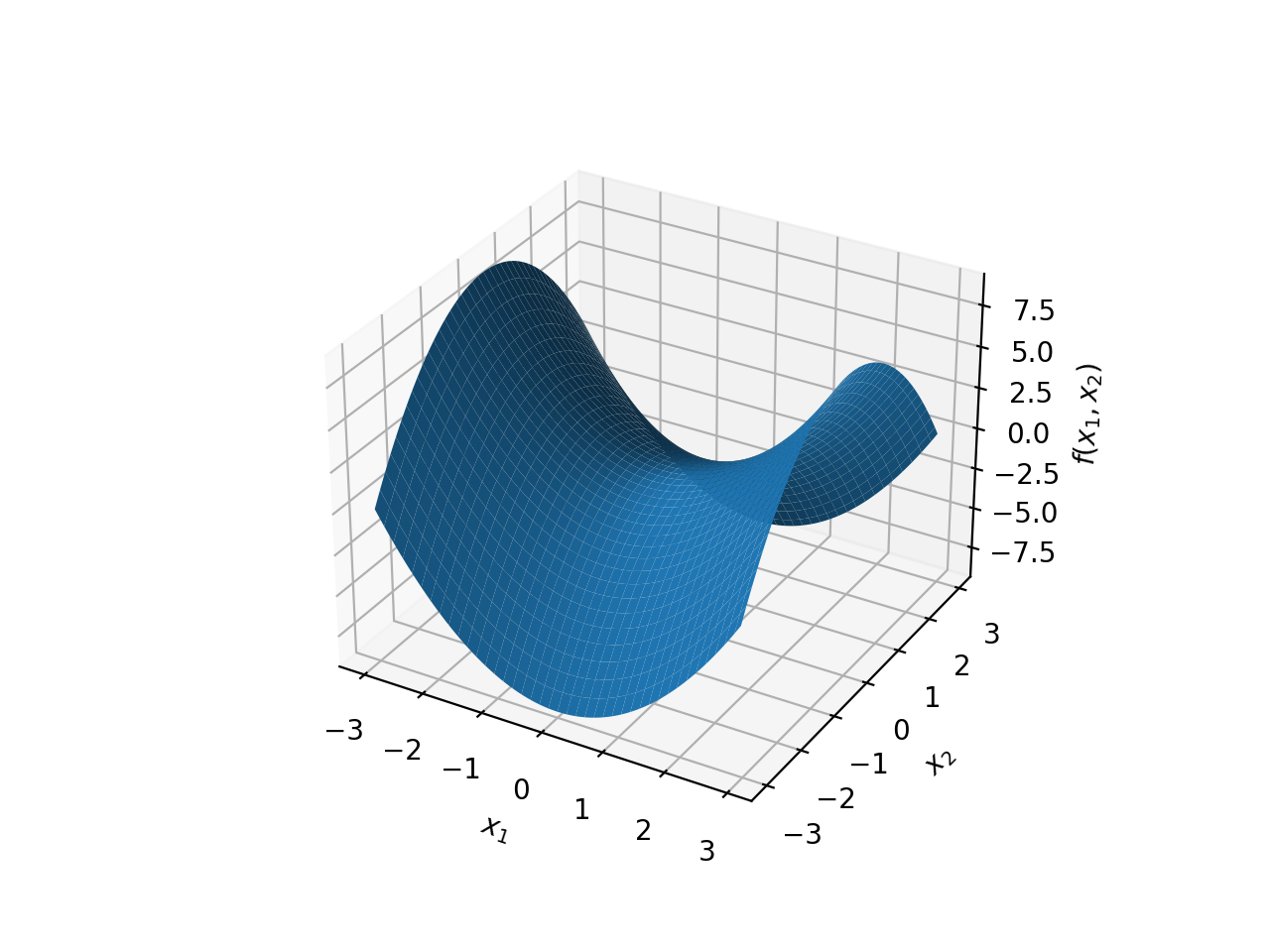
The above conditions also imply the existence of a saddle point in the solution space, which, as we will discuss, will also be the optimal solution.

---