The Gram-Schmidt Orthogonalisation

Avishek Sen Gupta on 27 May 2021

---

We discuss an important factorisation of a matrix, which allows us to convert a linearly independent but non-orthogonal basis to a linearly independent orthonormal basis. This uses a procedure which iteratively extracts vectors which are orthonormal to the previously-extracted vectors, to ultimately define the orthonormal basis. This is called the Gram-Schmidt Orthogonalisation, and we will also show a proof for this.

Projection of Vectors onto Vectors

This section derives the decomposition of a vector into two orthogonal components. These orthogonal components aren’t necessarily the standard basis vectors (\(\text{[1 0]}\) and \(\text{[0 1]}\) in \(\mathbb{R}^2\), for example); but they are guaranteed to be orthogonal to each other.

Assume we have the vector \(\vec{x}\) that we wish to decompose into two orthogonal components. Let us choose an arbitrary vector \(\vec{u}\) as one of the components; we will derive its orthogonal counterpart as part of this derivation.

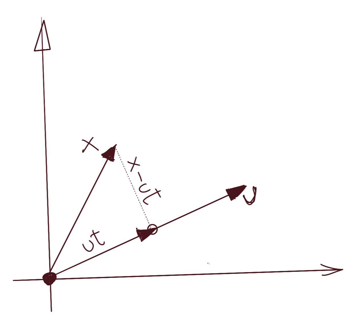
Since the projection will be collinear with \(\vec{u}\), let us assume the projection is \(t\vec{u}\), where \(t\) is a scalar. The only constraint we wish to express is that the vector \(\vec{u}\) and the plumb line from the tip of the vector \(\vec{x}\) to \(\vec{u}\) are perpendicular, i.e., their dot product is zero. We can see from the above diagram that the plumb line is \(\vec{x}-t\vec{u}\). We can then write:

\[u^T.(x-ut)=0 \\ \Rightarrow u^Tx=u^Tut \\ \Rightarrow t={(u^Tu)}^{-1}u^Tx\]

We know that \(u^Tu\) is the dot product of \(\vec{u}\) with itself, and thus a scalar, so you could write it as:

\[t=\frac{u^Tx}{u^Tu}\]

and indeed, we’d be justified in doing that, but let’s not make that simplification, because there is a more general case coming up, where this will not be a scalar. Thus, the component of \(\vec{x}\) in the direction \(\vec{u}\) is \(ut={(u^Tu)}^{-1}u^Txu\) and the orthogonal component will be \(x-ut=x-{(u^Tu)}^{-1}u^Txu\).

The one important thing to note is the expression for \(t\) in the general case, i.e., when it is not a scalar. It is basically the expression for the left inverse of a general matrix:

There is one simplifying assumption we can make: if \(\vec{u}\) is a unit vector, then \(u^Tu=I\), which simplifies the expressions to:

\[\mathbf{x_{u\parallel}={(u^Tu)}^{-1}u^Txu} \\ x_{u\parallel}=u^Txu \text{ (if u is a unit vector)}\\ \mathbf{x_{u\perp}=x-{(u^Tu)}^{-1}u^Txu} \\ x_{u\perp}=x-u^Txu \text{ (if u is a unit vector)}\]

Projection of Vectors onto Vector Subspaces

The same logic applies when we are projecting vectors onto vector subspaces. We use the same constraint, i.e.:

\[u^T.(x-ut)=0\]

There are a few differences in the meaning of the symbols worth noting. \(u\) is no longer a single column vector; it is a set of column vectors which define a vector subspace. Let’s assume the vector subspace is embedded in \(\mathbb{R}^n\), and we have \(m\) linearly independent vectors in \(u\) (\(m\leq n\)). \(u\) now becomes a \(n\times m\) matrix.

The projection is no longer gotten from scaling a single vector; it is now expressible as a linear combination of these \(m\) vectors. This set of weightings is \(t\), which now becomes a \(m\times 1\) matrix. This change of \(t\) from a scalar to a \(m\times 1\) matrix is also the reason we didn’t simplify the \(u^Tu\) expression in the previous section; in the general case, \(t\) is not a scalar.

\(\vec{x}\) is still an \(n\times 1\) matrix; this hasn’t changed.

Thus, the results of projection of a vector onto a vector subspace are still the same.

\[\mathbf{x_{u\parallel}={(u^Tu)}^{-1}u^Txu} \\ x_{u\parallel}=u^Txu \text{ (if u is a unit vector)}\\ \mathbf{x_{u\perp}=x-{(u^Tu)}^{-1}u^Txu} \\ x_{u\perp}=x-u^Txu \text{ (if u is a unit vector)}\] \[t={(u^Tu)}^{-1}u^Tx\]

Gram-Schmidt Orthogonalisation

We are now in a position to describe the intuition behind Gram-Schmidt Orthogonalisation. Let us state the key idea first.

For a set of \(m\) linearly independent vectors in \(\mathbb{R}^n\) which span some subspace \(V_m\), there exists aset of \(m\) orthonormal basis vectors, which span the same subspace \(V_m\).

The procedure goes as follows:

Assume \(m\) linearly independent (but not orthogonal) vectors in \(\mathbb{R}^n\). They span some subspace \(V_m\) of dimensionality \(m\). Let these vectors be \(x_1\), \(x_2\), \(x_3\), …, \(x_m\).

• We have to start somewhere, so let’s assume that our first orthogonal basis vector is \(u_1=\frac{x_1}{\|x_1\|}\) (normalise to be a unit vector). \(u_1\) is our first orthogonal basis vector.
• We now project \(x_2\) onto \(u_1\), finding \({x_2}_{u_1\parallel}\) and \({x_2}_{u_1\perp}\) as we have described in the previous sections. We won’t really use \({x_2}_{u_1\parallel}\) except to calculate its orthogonal component \({x_2}_{u_1\perp}\).

• Designate \(u_2={x_2}_{u_1\perp}\). Because of the way we have constructed \(u_2\), \(u_2\) is orthogonal to \(u_1\). We now have two orthogonal basis vectors, \(u_1\), \(u_2\). Normalise them to unit vectors as needed. Computationally, \(u_2\) looks like this:

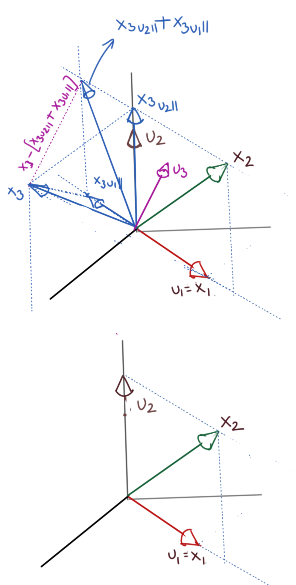
  \[u_2=x_2-{u_1}^Tx_{2}u_1\]
• Now let us project \(x_3\) onto \(u_1\) and \(u_2\) to get \(({x_3}_{u_1\parallel}, {x_3}_{u_2\parallel})\). Calculate \({x_3}_{u_1,u_2\perp}=x_3-{x_3}_{u_1\parallel}-{x_3}_{u_2\parallel}\).

• Designate \(u_3={x_3}_{u_1,u_2\perp}\). We now have three orthogonal basis vectors, \(u_1\), \(u_2\), \(u_3\). Normalise them to unit vectors as needed. Computationally, \(u_3\) looks like this:

  \[u_2=x_3-{u_1}^Tx_{3}u_1-{u_2}^Tx_{3}u_2\]
• Repeat the above procedure for all the remaining vectors upto \(x_m\). At the end, we will have \(m\) orthogonal basis vectors \((u_1, u_2, ..., u_m)\) which will span the same vector subspace \(V_m\).

You will notice that at every stage of this procedure, the next orthogonal basis vector to be computed, is given by the following general identity:

\[u_{k+1}=x_{k+1}-\sum_{i=1}^{k}{u_i}^Tx_{k+1}u_i\]

It is very easy to see that at every step, the latest basis vector is orthogonal to every other previously-generated basis vector. To see this, take the dot product on both sides with an arbitrary \(u_j\), such that \(j\leq k\).

\[{u_j}^Tu_{k+1}={u_j}^Tx_{k+1}-\sum_{i=1}^{k}{u_j}^T\underbrace{ ({u_i}^Tx_{k+1}) }_{scalar}u_i \\ ={u_j}^Tx_{k+1}-\sum_{i=1}^{k}\underbrace{ ({u_i}^Tx_{k+1}) }_{scalar}{u_j}^Tu_i\]

Because of the way we have constructed the previous orthogonal basis vectors, we have \({u_j}^Tu_i=0\) for all \(j\neq i\), and \({u_j}^Tu_i=1\) for \(j=i\) (assuming unit basis vectors). Thus, the above identity becomes:

\[{u_j}^Tu_{k+1}={u_j}^Tx_{k+1}-{u_j}^Tx_{k+1}=0\]

Proof of Gram-Schmidt Orthogonalisation

A very valid question is: why does the basis from the Gram-Schmidt procedure span the same vector subspace as the one spanned by the original non-orthogonal basis?

The proof should make this clear; most of it follows almost directly from the procedure itself; we only need to fill in a few gaps, and formalise the presentation.

Given a set of \(m\) linearly independent vectors \((x_1, x_2, x_3, ..., x_m)\) in \(\mathbb{R}^n\) spanning a vector subspace \(V\in\mathbb{R}^m\), there exists an orthogonal basis \((u_1, u_2, u_3, ..., u_m)\) which spans the vector subspace \(V\in\mathbb{R}^m\).

We prove this by induction.

1. Proof for \(n=1\)

Let us validate the hypothesis for \(n=1\). For \(x_1\), if we take \(u_1=\frac{x_1}{\|x_1\|}\), we can see that \(u_1\) spans the same vector subspacee as \(x_1\), since it’s merely a scaled version of \(x_1\).

2. Proof for \(n=k+1\)

Let us now assume that the above statement holds for \(n=k\leq m\), i.e., there are \(k\) orthogonal basis vectors \((u_1, u_2, u_3, ..., u_k)\) which span the same vector subspace \(V\in\mathbb{R}^k\) as the set \((x_1, x_2, x_3, ..., x_k)\).

Now, consider the construction of the \((k+1)\)th orthogonal basis vector \(u_{k+1}\) like so:

\[u_{k+1}=x_{k+1}-\sum_{i=1}^{k}{u_i}^Tx_{k+1}u_i\]

It is very easy to see that at every step, the latest basis vector is orthogonal to every other previously-generated basis vector. To see this, take the dot product on both sides with an arbitrary \(u_j\), such that \(j\leq k\).

\[{u_j}^Tu_{k+1}={u_j}^Tx_{k+1}-\sum_{i=1}^{k}{u_j}^T\underbrace{ ({u_i}^Tx_{k+1}) }_{scalar}u_i \\ ={u_j}^Tx_{k+1}-\sum_{i=1}^{k}\underbrace{ ({u_i}^Tx_{k+1}) }_{scalar}{u_j}^Tu_i\]

Because of the way we have constructed the previous orthogonal basis vectors, we have \({u_j}^Tu_i=0\) for all \(j\neq i\), and \({u_j}^Tu_i=1\) for \(j=i\) (assuming unit basis vectors). Thus, the above identity becomes:

\[{u_j}^Tu_{k+1}={u_j}^Tx_{k+1}-{u_j}^Tx_{k+1}=0\]

Thus, the newly constructed basis vector is orthogonal to every basis vector \((u_1, u_2, u_3, ..., u_k)\). This completes the induction part of the proof.

3. Proof that \(u_{k+1}\neq 0\)

We also prove that the newly-constructed basis vector is not a zero vector. For that, let us assume that \(u_{k+1}=0\). Then, we get:

\[x_{k+1}-\sum_{i=1}^{k}{u_i}^Tx_{k+1}u_i=0 \\ x_{k+1}=\sum_{i=1}^{k}{u_i}^Tx_{k+1}u_i\]

This implies that \(x_{k+1}\) is expressible as a linear combination of the set of vectors \((u_1, u_2, u_3, ..., u_k)\). But we have also assumed that this set spans the same vector subspace as \((x_1, x_2, x_3, ..., x_k)\).

This implies that \(x_{k+1}\) is expressible as a linear combination of the set \((x_1, x_2, x_3, ..., x_k)\), which is a contradiction, since the vectors in the full set \((x_1, x_2, x_3, ..., x_m)\) are linearly independent. Thus, \(u_{k+1}\) cannot be zero.

\[\blacksquare\]

---