This article lays the groundwork for an important construction called Reproducing Kernel Hilbert Spaces, which allows a certain class of functions (called Kernel Functions) to be a valid representation of an inner product in (potentially) higher-dimensional space. This construction will allow us to perform the necessary higher-dimensional computations, without projecting every point in our data set into higher dimensions, explicitly, in the case of Non-Linear Support Vector Machines, which will be discussed in the upcoming article.
This construction, it is to be noted, is not unique to Support Vector Machines, and applies to the general class of techniques in Machine Learning, called Kernel Methods. An important part of the construction relies on defining the inner product of functions, as well as notions of Positive Semi-Definiteness: these are the concepts we will discuss in this article.
A lot of this material stems from Functional Analysis, and we will attempt to introduce the relevant material here as painlessly as possible for the engineer.
Most of the ideas here can be intuitively related to familiar notions of \(\mathbb{R}^n\) spaces, and we’ll use motivating examples to connect the mathematical machinery to the engineer’s intuition.
Motivation for Kernel Functions
We begin with the motivation for introducing this material. Consider a set of ten data points, all one-dimensional. We write them as:
\[x_1, x_2, x_3, ..., x_10\in\mathbf{R}\]Furthermore, let us assume that some of them belong to the class Green, and the rest to the class Red. Let us assign values and classes to them, to be more concrete:
| \(x_1\) | \(x_2\) | \(x_3\) | \(x_4\) | \(x_5\) | \(x_6\) | \(x_7\) | \(x_8\) | \(x_9\) | \(x_{10}\) |
|---|---|---|---|---|---|---|---|---|---|
| -5 | -4 | -3 | -2 | -1 | 0 | 1 | 2 | 3 | 4 |
| Red | Red | Red | Green | Green | Green | Green | Green | Red | Red |
We represent them on the number line, like so

Our aim is to find a linear partitioning line which separates all the Green points from all the Red sets. Note that this linear partitioning “line” is called different names in different dimensions, the common term being the separating hyperplane:
- A point in \(\mathbb{R}\)
- A line in \(\mathbb{R}^2\)
- A plane in \(\mathbb{R}^3\)
In this case, we would like to find a single point that creates a Red and a Green partition.
You can quickly see that there is no way you can choose a single point that can do this. This is obviously because the Green data set is “surrounded” by the Red data set on either side.
There is a way out of this quandary: we can lift our original data set into a higher dimension. As an illustration, let us pick the function \(f(x)=x^2\) to lift our data set into \(\mathbb{R}^2\).
Our data set now becomes:
| \(x_1\) | \(x_2\) | \(x_3\) | \(x_4\) | \(x_5\) | \(x_6\) | \(x_7\) | \(x_8\) | \(x_9\) | \(x_{10}\) |
|---|---|---|---|---|---|---|---|---|---|
| -5 | -4 | -3 | -2 | -1 | 0 | 1 | 2 | 3 | 4 |
| 25 | 16 | 9 | 4 | 1 | 0 | 1 | 4 | 9 | 16 |
| Red | Red | Red | Green | Green | Green | Green | Green | Red | Red |
Now, can we separate the resulting two-dimensional points using a linear function? Yes, we can. I’ve picked a random straight line \(x-2y+12=0\) to illustrate this separation, but there is an infinite number of straight lines that will do the work. This situation is shown below:
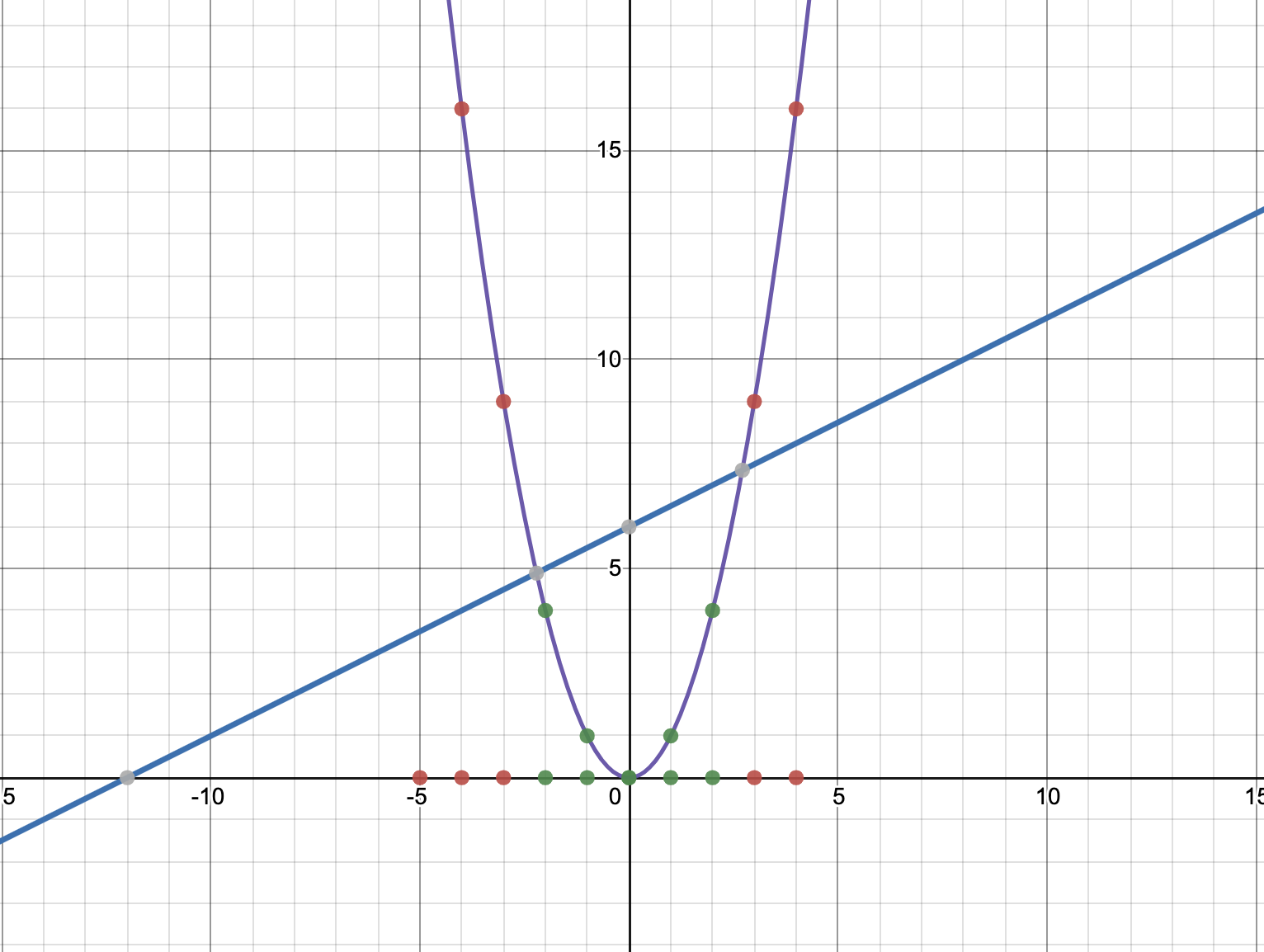
You could have lifted this same data set to \(\mathbb{R}^3\), \(\mathbb{R}^4\), etc. as well, but in this particular case, lifting it to \(\mathbb{R}^2\) makes it nicely linearly separable, so we don’t need to go higher.
The same concept applies to higher dimensional data sets. A linearly non-separable data set in \(\mathbb{R}^2\) can be made linearly separable (using a plane) if it is lifted to \(\mathbb{R}^3\).
This is a common technique used in Machine Learning algorithms as a way to make classification problems easier. Generally speaking, a linearly non-separable data set can be made linearly separable by projecting it onto a higher dimension. This projection into higher dimensions is not an ML algorithm by itself, but can be an important step as part of data preparation.
This by itself is not the problem. As we will see later on, Machine Learning algorithms tend to perform the inner product operation very frequently. This inner product needs to be performed on thousands (if not millions) of data points, each of which need to be lifted to a higher dimension, before the inner product operation can be carried out.
We ask the following question: when is a function on a pair of original vectors also the inner product of those vectors projected into a higher dimensional space? If we can answer this question, then we can circumvent the process of projecting a pair of vectors into higher-dimensional space, and then computing their inner products; we can simply apply a single function which gives us the inner products in higher dimensional space.
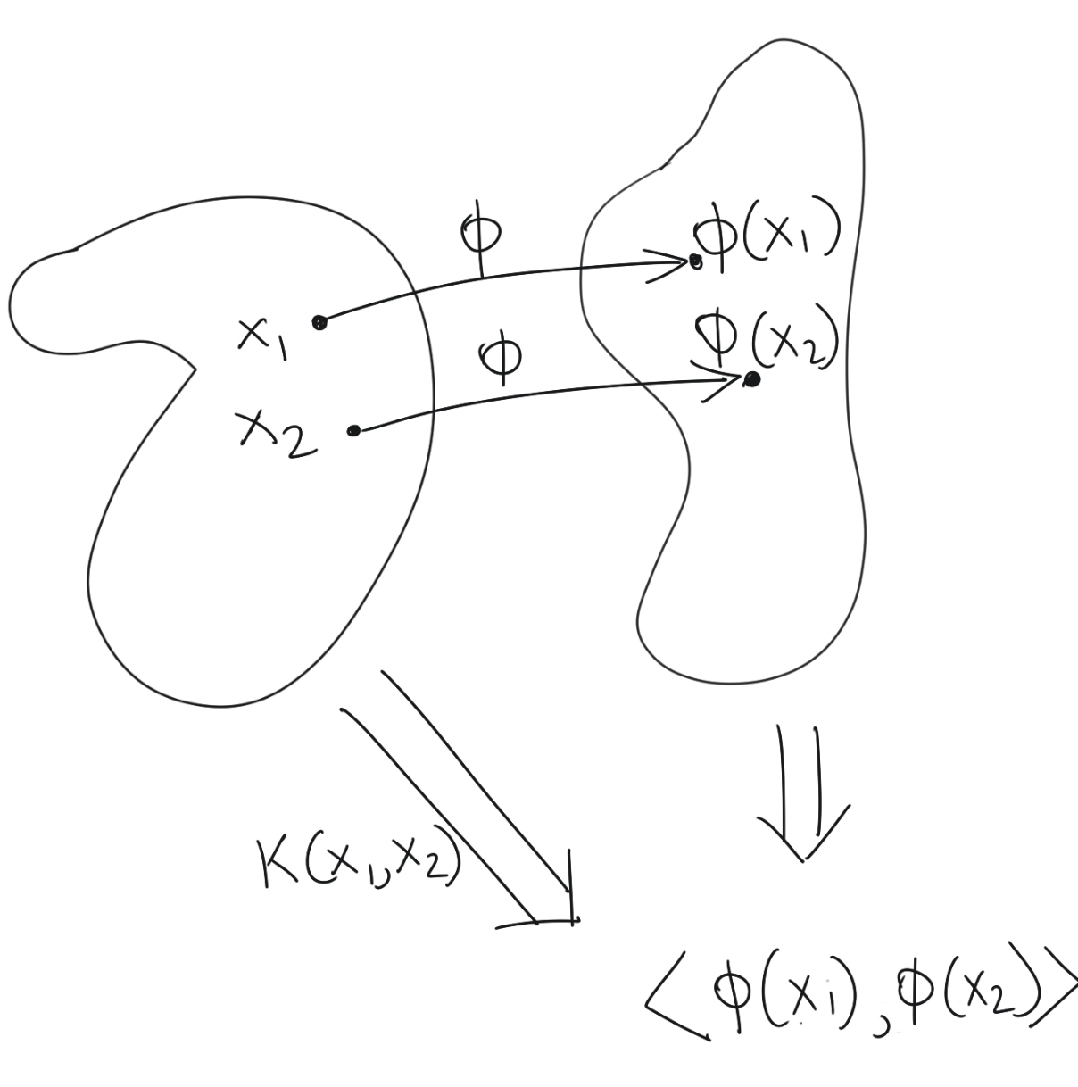
Such a function which satisfies our requirements is called a Kernel Function, and is the main motivation for developing the mathematical preliminaries in this article.
Mathematical Preliminaries
Functions as Infinite-Dimensional Vectors
We can treat functions as vectors. Indeed, this is one of the unifying ideas behind Functional Analysis. A proper treatment of this concept can be found in any good Functional Analysis text, but I will introduce the relevant concepts here.
We are used to dealing with finite dimensional vectors, mostly in \(\mathbb{R}^n\). A function \(f:\mathbb{R}^n\rightarrow \mathbb{R}\) in the most general sense, can be treated as a sequence of vectors. However, even if we restrict the domain of a function, there is always an infinite number of values that the function \(f\) will take within even this restricted domain, since there are always going to be an infinite number of real numbers in the chosen interval.
We can proceed to build our intuition by looking at the following arbitrary function. For convenience of discussion, we restrict the discussion to the range \(x\in[a,b]\).
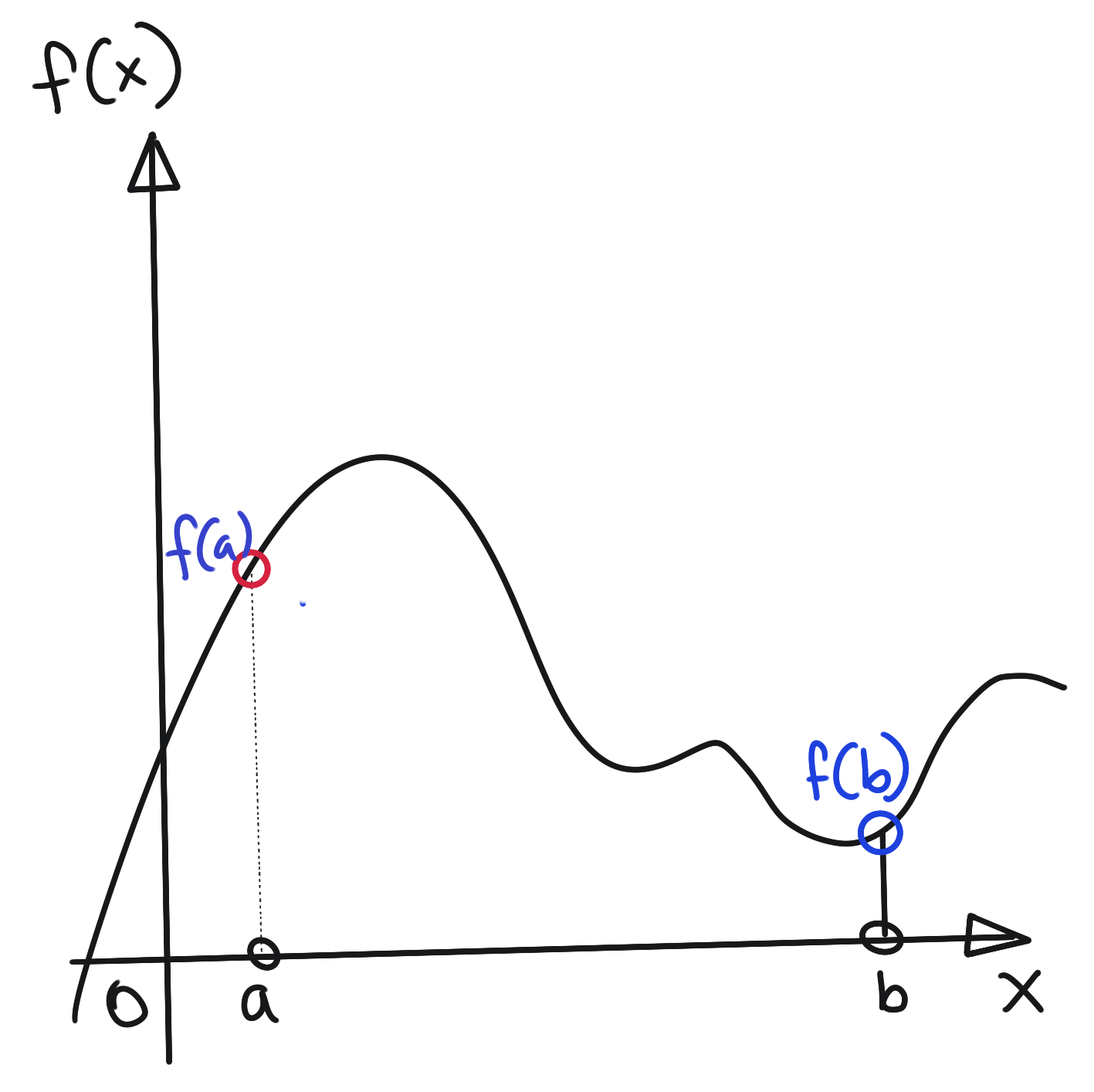
Let us decide to approximate this function \(f(x)\) by taking five samples at equal intervals \(\Delta x\), as below:
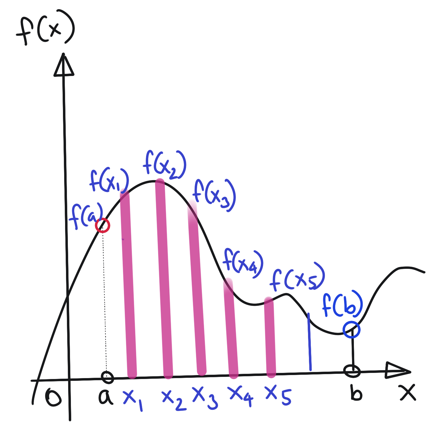
We may represent this approximation of \(f(x)\) by a vector of these five samples, i.e.,
\[\tilde{f}(x)=\begin{bmatrix} f(x_1) \\ f(x_2) \\ f(x_3) \\ f(x_4) \\ f(x_5) \end{bmatrix}\]The above is a vector in \(\mathbb{R}^5\). Increasing the number of samples (which in turn decreases \(\Delta x\)), results in a higher dimensional vector, as shown below:
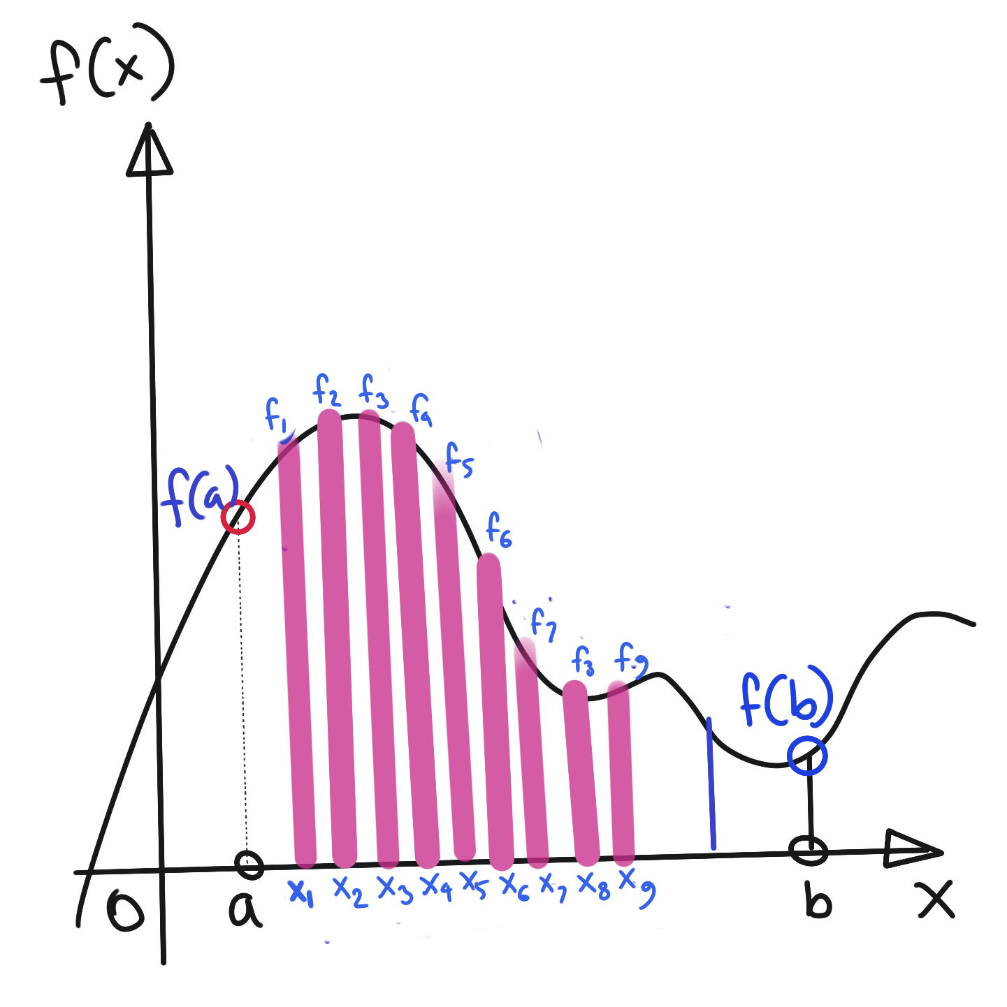
Now, we can approximate \(f(x)\) with a 9-dimensional vector, like so:
\[\tilde{f}(x)=\begin{bmatrix} f_1 \\ f_2 \\ f_3 \\ f_4 \\ f_5 \\ f_6 \\ f_7 \\ f_8 \\ f_9 \end{bmatrix}\]Clearly, the higher the dimensionality of our approximating vector, the better the approximation to the original function. Ultimately, as \(n\rightarrow \infty\), and \(\Delta x\rightarrow 0\), we recover the true function, and the “approximating vector” is now infinite-dimensional. However, the infinite dimensionality does not prevent us from performing usual vector algebra operations on this function.
Indeed, we can show that functions respect all the axioms of a vector space, that is:
- The operations of Vector Addition and Scalar Multiplication are valid for functions.
- Commutativity of Addition: \(a+b=b+a\)
- Associativity of Addition: \(a+(b+c)=(a+b)+c\)
- Existence of Additive Identity: \(a+0=a\)
- Existence of Additive Inverse: \(a+(-a)=0\)
- Existence of Multiplicative Identity: \(a.1=a\)
- Distributivity of Scalar Multiplication with respect to Vector Addition: \(\alpha\cdot(a+b)=\alpha\cdot a + \alpha\cdot b\)
- Distributivity of Scalar Multiplication with respect to Field Addition: \((\alpha + \beta)\cdot a=\alpha\cdot a + \beta\cdot a\)
Hilbert Spaces
There is one important property of vector spaces that we’ve taken for granted in our discussions on Linear Algebra so far: the fact that the inner product is a defined operation in our \(\mathbb{R}^n\) Euclidean space.
The Dot Product that I’ve covered in previous posts with reference to Linear Algebra is essentially a specialisation of the general concept of the Inner Product applied to finite-dimensional Euclidean spaces. We will begin using the more general term Inner Product in further discussions.
Another important point to note: we will be switching up notation. Inner products will henceforth be designated as \(\langle\bullet,\bullet\rangle\). Thus, the inner product of two vectors \(x\) and \(y\) will be written as \(\langle x,y\rangle\).
The inner product is not defined on a vector space by default: the property must be explicitly stated as valid on a vector space. A vector space equipped with an inner product operation is formally known as a Hilbert space. Thus, the vector spaces we have been dealing with in Linear Algebra so far, have necessarily been Hilbert spaces.
There are a few important properties any candidate for an inner product must satisfy. All these properties intuitively make sense since we’ve been using them without stating them implicitly while doing Matrix Algebra.
- Positive Definite: \(\langle x,x\rangle>0\) if \(x\neq 0\)
- Principle of Indiscernibles: \(x=0\) if \(\langle x,x\rangle=0\)
- Symmetric: \(\langle x,y\rangle=\langle y,x\rangle\)
- Linear:
- \[\langle \alpha x,y\rangle=\alpha\langle x,y\rangle, \alpha\in\mathbb{R}\]
- \[\langle x+y,z\rangle=\langle x,z\rangle+\langle y,z\rangle\]
Norm induced by Inner Product
Another interesting property we have taken for granted is the existence of the norm of a vector \(\|\bullet\|\). In plain Linear Algebra, the norm is essentially the magnitude of a vector. What is interesting is that the norm need not be separately specified as a property of vector space; it comes into existence automatically if an inner product is defined on a vector space. To see why this is the case, note that:
\[\langle x,x\rangle=\|x\|^2 \\ \Rightarrow \|x\|=\sqrt{\langle x,x\rangle}\]Inner Product of Functions
Since the vector space of functions is also a Hilbert space, we should be able to take the inner product of two functions. Here’s some intuition about what the inner product of functions actually means, and how it comes into being.
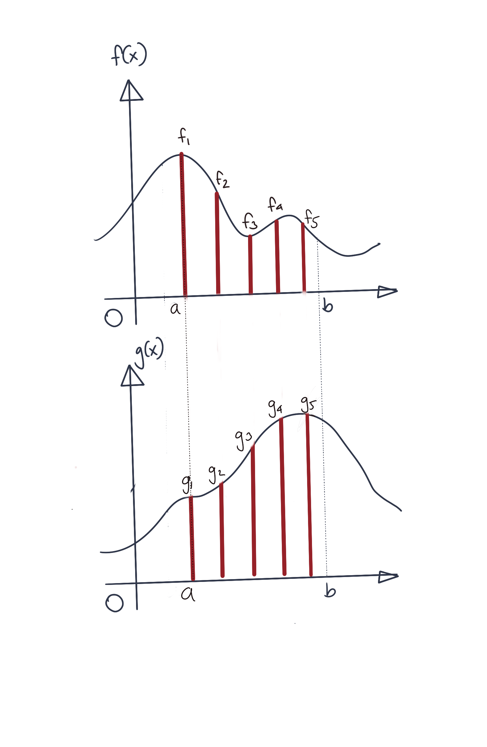
We will begin by assuming some approximation of two functions \(f\) and \(g\) using finite-dimensional vectors. For concreteness’ sake, assume we represent them using 5-dimensional vectors. We have represented the approximating vectors \(\tilde{f}\) and \(\tilde{g}\), like so:
\[\tilde{f}(x)=\begin{bmatrix} f_1 \\ f_2 \\ f_3 \\ f_4 \\ f_5 \end{bmatrix} \tilde{g}(x)=\begin{bmatrix} g_1 \\ g_2 \\ g_3 \\ g_4 \\ g_5 \end{bmatrix}\]As usual, we have restricted the domain of discussion to be \([a,b]\). Also note that
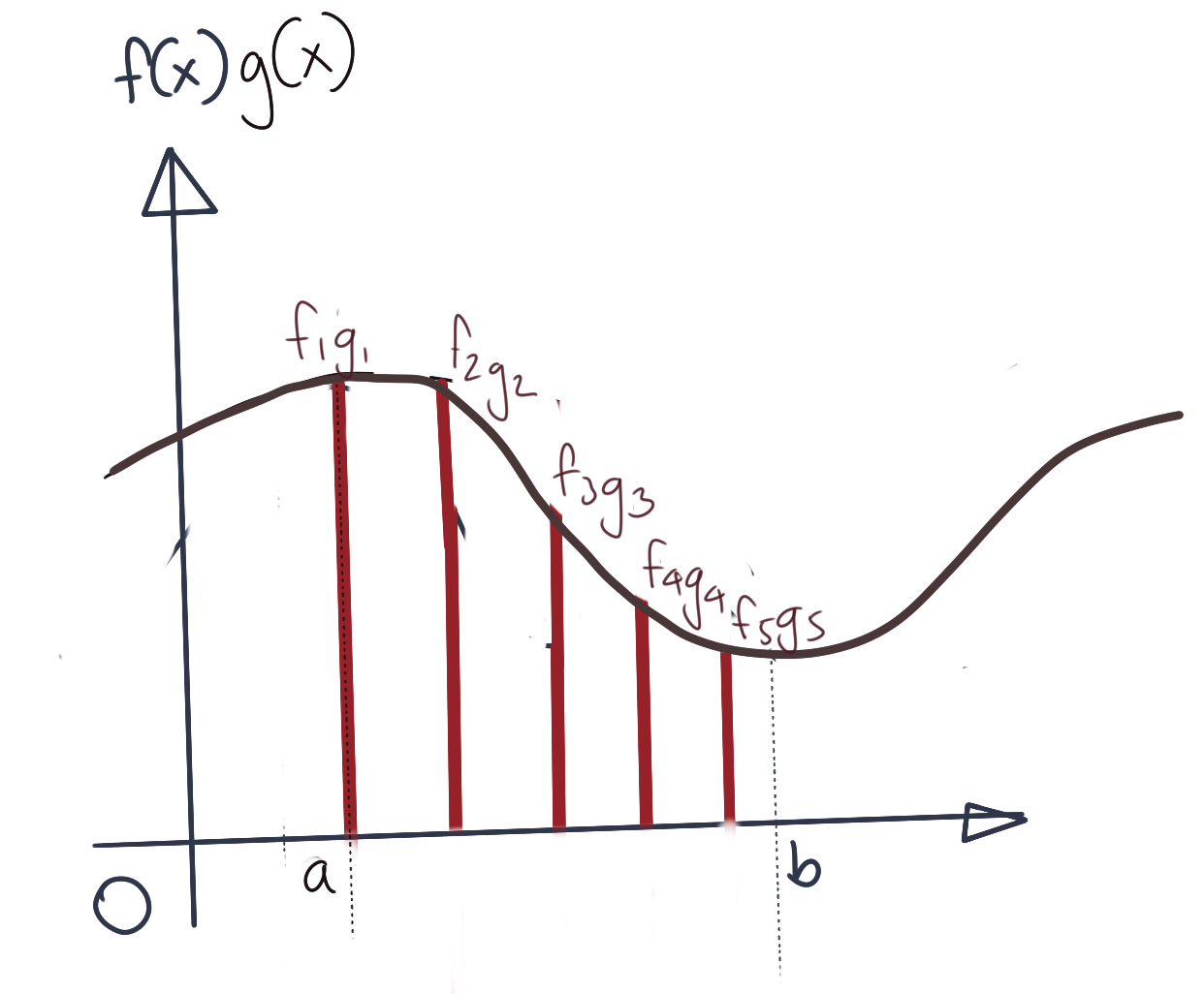
The approximate vector after multiplying the coefficients in the corresponding dimensions would then be:
\[\tilde{f(x)}\tilde{g(x)}=\begin{bmatrix} f_1.g_1 \\ f_2.g_2 \\ f_3.g_3 \\ f_4.g_4 \\ f_5.g_5 \end{bmatrix}\]Note that the above vector is not the actual inner product, for that we will still need to sum up the samples as we describe next. Let us assume that if the inner product \(\langle f,g\rangle\) was computed perfectly, it would have the graph as below. Here the true inner product is shown along with the vector \(\tilde{f(x)}\tilde{g(x)}\) overlaid onto it.
Now let us consider how you’d want to calculate the inner product. Naively, we can simply sum up the values of \(\tilde{f(x)}\tilde{g(x)}\). However, this would not necessarily be a good approximation, since we are leaving out parts of the function that we are not sampling. All the parts of the function between any consecutive pair of samples are not accounted for at all. How are we then to approximate these missing values.
In the absence of further data, the best we can do is assume that those missing values are the same as the value of the sample immediately preceding them. Essentially, to compute the approximation for the missing parts of the function, we need to compute the area of the approximating rectangle, the height of which is the value of the immediately preceding sample. The approximation is as shown below.
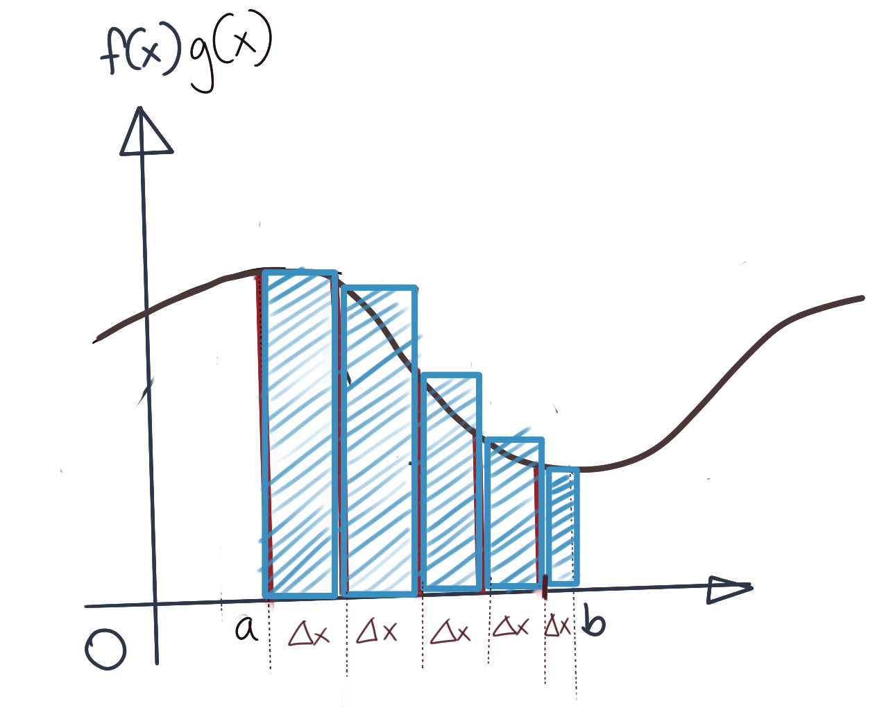
Thus, the approximate inner product \({\langle f,g\rangle}_{approx}\) is:
\[{\langle f,g\rangle}_{approx}=\sum_{i=1}^N f_i\cdot g_i\cdot\Delta x\]Of course, this is only an approximation, and the more samples we take, the better our approximation will be. In the limit where \(\Delta x\rightarrow 0\), and \(i\rightarrow\infty\), this changes into an integral with limits \(a\) and \(b\), as below:
\[{\langle f,g\rangle}=\int_a^b f(x)g(x)dx\]Thus, the inner product of two functions is the area under the product of the two functions.
Functions as Basis Vectors
If functions can be treated as vectors, we should be able to express - and create - functions as linear combinations of other functions. The implication then is also that functions can also serve as basis vectors. We can essentially bring to bear all the machinery of Linear Algebra, since its results apply to all sorts of vectors. Things like orthogonality, projections, etc. also apply to functions now. The unifying idea is that vectors can be matrices, or functions, or other things.
Thus, a set of functions can span a vector space of functions. This idea will be an important part in the construction of RKHS’s.
Postive Semi-Definite Kernels and the Gram Matrix
Positive semi-definite matrices are square symmetric matrices which have the following property:
\[v^TSv\geq 0\]where \(S\) is the \(n\times n\) matrix, and \(v\) is a \(n\times 1\) vector. You can convince yourself that the final result of \(v^TSv\) is a single scalar.
Positive semi-definite matrices can always be expressed as the product of a matrix and its transpose.
\[A=L^TL\]See Cholesky and \(LDL^T\) Factorisations for further details on how this decomposition works. To see why a Cholesky-decomposable matrix satisfies the positive semi-definiteness property, rewrite \(v^TSv\) so that:
\[v^TSv=v^TL^TLv \\ =(v^TL^T)(Lv) \\ ={(Lv)}^T(Lv) ={\|Lv\|}^2 \geq 0\]The important result to know is that all positive semi-definite matrices have a Cholesky Factorisation. We will explore the proof in a future post.
Inner Product and the Gram Matrix
With this intuition, we turn to a common operation in many Machine Learning algorithms: the Inner Product. The inner product is a very common operation. As we discussed in the first section of this article, inner product calculations usually need to be combined with projecting the original input vectors to a higher dimensional space first. We will revisit the SVM equations in an upcoming post to see the use of the Gram Matrix, which in the context of kernel functions is simply the matrix of all possible inner products of all data points.
Assume we have \(n\) data vectors \(x_1\), \(x_2\), \(x_3\), …, \(x_n\). The matrix that will be used to characterise the positive semi-definiteness of kernels is called the Gram Matrix. Given \(n\) data points \(x_1\), \(x_2\), …, \(x_n\), the Gram matrix is written as:
\[K=\begin{bmatrix} \kappa(x_1, x_1) && \kappa(x_2, x_1) && ... && \kappa(x_n, x_1) \\ \kappa(x_1, x_2) && \kappa(x_2, x_2) && ... && \kappa(x_n, x_2) \\ \kappa(x_1, x_3) && \kappa(x_2, x_3) && ... && \kappa(x_n, x_3) \\ \vdots && \vdots && \ddots && \vdots \\ \kappa(x_1, x_n) && \kappa(x_2, x_n) && ... && \kappa(x_n, x_n) \\ \end{bmatrix}\]where \(\kappa(x,y)\) is the kernel function. We will say that the kernel function is positive semi-definite if:
\[v^TKv\geq 0\]where \(v\) is any \(n\times 1\) vector. Let’s expand out the final result because that is a form we will see in both the construction of the Reproducing Kernel Hilbert Spaces, as well as the solutions for Support Vector Machines.
Let \(v=\begin{bmatrix} \alpha_1 \\ \alpha_2 \\ \vdots \\ \alpha_n \\ \end{bmatrix}\)
Then, expanding everything out, we got:
\[v^TKv= \begin{bmatrix} \alpha_1 && \alpha_2 && \ldots && \alpha_n \end{bmatrix} \cdot \begin{bmatrix} \kappa(x_1, x_1) && \kappa(x_2, x_1) && ... && \kappa(x_n, x_1) \\ \kappa(x_1, x_2) && \kappa(x_2, x_2) && ... && \kappa(x_n, x_2) \\ \kappa(x_1, x_3) && \kappa(x_2, x_3) && ... && \kappa(x_n, x_3) \\ \vdots && \vdots && \ddots && \vdots \\ \kappa(x_1, x_n) && \kappa(x_2, x_n) && ... && \kappa(x_n, x_n) \\ \end{bmatrix} \cdot \begin{bmatrix} \alpha_1 \\ \alpha_2 \\ \vdots \\ \alpha_n \\ \end{bmatrix} \\= {\begin{bmatrix} \alpha_1\kappa(x_1, x_1) + \alpha_2\kappa(x_1, x_2) + \alpha_3\kappa(x_1, x_3) + ... + \alpha_n\kappa(x_1, x_n) \\ \alpha_1\kappa(x_2, x_1) + \alpha_2\kappa(x_2, x_2) + \alpha_3\kappa(x_2, x_3) + ... + \alpha_n\kappa(x_2, x_n) \\ \alpha_1\kappa(x_3, x_1) + \alpha_2\kappa(x_3, x_2) + \alpha_3\kappa(x_3, x_3) + ... + \alpha_n\kappa(x_3, x_n) \\ \vdots \\ \alpha_1\kappa(x_n, x_1) + \alpha_2\kappa(x_n, x_2) + \alpha_3\kappa(x_n, x_3) + ... + \alpha_n\kappa(x_n, x_n) \\ \end{bmatrix}}^T \cdot \begin{bmatrix} \alpha_1 \\ \alpha_2 \\ \vdots \\ \alpha_n \\ \end{bmatrix} \\= {\begin{bmatrix} \sum_{i=1}^n\alpha_i\kappa(x_1, x_i) \\ \sum_{i=1}^n\alpha_i\kappa(x_2, x_i) \\ \sum_{i=1}^n\alpha_i\kappa(x_3, x_i) \\ \vdots \\ \sum_{i=1}^n\alpha_i\kappa(x_n, x_i) \\ \end{bmatrix}}^T \cdot \begin{bmatrix} \alpha_1 \\ \alpha_2 \\ \vdots \\ \alpha_n \\ \end{bmatrix} \\ = \alpha_1\sum_{i=1}^n\alpha_i\kappa(x_1, x_i) +\alpha_2\sum_{i=1}^n\alpha_i\kappa(x_2, x_i) +\alpha_3\sum_{i=1}^n\alpha_i\kappa(x_3, x_i) +\ldots +\alpha_n\sum_{i=1}^n\alpha_i\kappa(x_n, x_i) \\ = \sum_{j=1}^n\sum_{i=1}^n\alpha_i\alpha_j\kappa(x_j, x_i)\]Note that the first factor in a couple of lines, is written in transpose form to make it more readable. Thus, from the above expansion, we get:
\[K=v^TKv=\sum_{j=1}^n\sum_{i=1}^n\alpha_i\alpha_j\kappa(x_j, x_i)\]For a positive semi-definite kernel \(K\), we must have this expression non-negative, that is:
\[\sum_{j=1}^n\sum_{i=1}^n\alpha_i\alpha_j\kappa(x_j, x_i) \geq 0\]