Statistics from Geometry and Linear Algebra

Avishek Sen Gupta on 12 August 2021

---

This article covers some common statistical quantities/metrics which can be derived from Linear Algebra and corresponding intuitions from Geometry, without recourse to Probability or Calculus. Of course, those subjects add more rigour and insight into these concepts, but our aim is to provide a form of intuitive shorthand for the reader.

Much of this stems from me attempting to understand links between statistical concepts and Linear Algebra. This post is a work in progress and will receive new additions over time.

We will discuss the following relations:

• Mean as the Projection Coefficient onto the Model Vector
• Variance as the Averaged Projection onto the Null Space of the Model Vector
• Pearson’s Correlation Coefficient as the Cosine of Angle between Two Vectors
• Linear Regression Coefficient as the Coefficient of Projection

Note on Convention

For data sets, we use the convention of observations-by-features. Each row in a matrix is a single point in the data set, i.e., an observation. A single column represents the sequence of recordings of a single feature (dimension) across all the points in our data set.

Accordingly, any data matrix will be an \(O\times F\) matrix, with \(O\) data points, and \(F\) dimensions.

Mean, covariance, etc. are always computed for a given dimension (feature), not across dimensions, which would make no sense, since each dimension represents a separate domain variable. In terms of probability, each feature is a Random Variable.

Mean as the Projection Coefficient onto the Model Vector

Assume \(n\) scalar observations which form a vector \(x\in\mathbb{R}^n\). This represents \(n\) data vectors in \(\mathbb{R}\). Then the mean of this set of observations is the projection of \(x\) onto the All-Ones Vector given by \(\nu_1\in\mathbb{R}^n\). We will refer to \(\nu_1\) as the Model Vector, going forward.

The Model Vector looks like:

\[\begin{bmatrix} 1 \\ 1 \\ \vdots \\ 1 \end{bmatrix} \Leftarrow n\text{ entries}\]

Recall that the projection coefficient of a vector \(b\) onto a vector \(a\) is given by:

\[\begin{equation} t=\frac{a^Tb}{a^Ta} \label{eq:projection-coefficient} \end{equation}\]

The situation is as below.

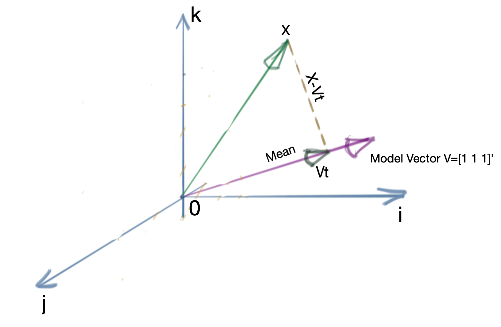
In this case, \(a=\nu_1\) and \(b=x\). Note that \(\nu_1^T\nu_1=n\), so we get:

\[t=\frac{\nu_1^Tb}{\nu_1^T\nu_1} \\ t=\frac{1}{n} \left( \begin{bmatrix} 1 && 1 && \cdots && 1 \end{bmatrix} \begin{bmatrix} x_1 \\ x_2 \\ \vdots \\ x_n \end{bmatrix} \right) \\ = \frac{x_1+x_2+\cdots+x_n}{n} \\ = \frac{1}{n}\sum_{i=1}^n x_i\]

which is the formula for the mean.

Notes

• In this geometric view, the mean is also a vector defined in terms of the Model Vector by \(\nu_1t\). This we will call the Mean Vector \(X_\mu\).
• It is important to note what the mean here represents: it is the mean vector of a set of \(n\) 1-dimensional vectors (\(\mathbb{R}\)).

Variance as the Averaged Projection onto the Null Space of the Model Vector

A similar relation holds for the variance of a data set. For the mean, we have already calculated the projection of the data set vector onto the Model Vector. The vector \(X-\nu_1t\) is, by definition, always perpendicular to the Model Vector \(\nu_1\), and thus lies in its null space.

In \(\mathbb{R}^n\) (for \(n\) entries in the data set), the nullspace of the Model Vector is the plane perpendicular to it and passing through the origin, as shown in the image below. Obviously, \(X-\nu_1t\) lies on this plane. This plane is referred to as the Error Space. Thus, stated another way,\(X-\nu_1t\) is the projection of the data vector \(X\) onto the nullspace of the Model Vector.

Of particular note is the fact that the Error Space is an \((n-1)\)-dimensional hyperplane in \(\mathbb{R}^n\). The variance is defined as the norm squared of the projection of the dataset vector \(X\) into the Error Space, averaged across a set of orthonormal basis vectors in the Error Space.

For an \((n-1)\)-dimensional hyperplane, the number of orthonormal basis vectors is \(n-1\). See the picture below for clarification.

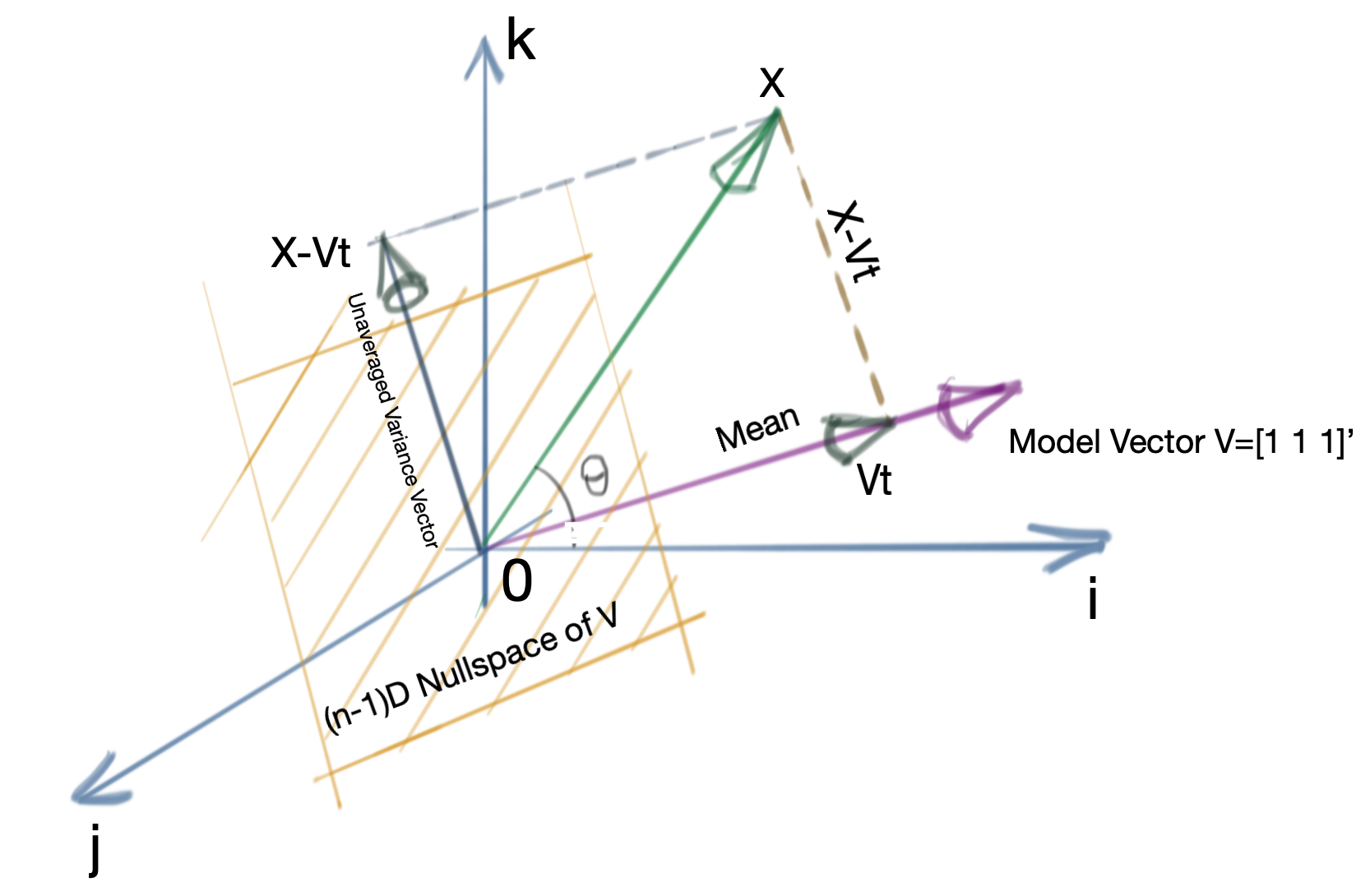
The variance then comes out as:

\[\begin{aligned} \sigma^2 &=\frac{ {\|X-X_\mu\|}^2}{n-1} \\ &\mathbf{=\frac{ {(X-X_\mu)}^T(X-X_\mu)}{n-1}}\\ &\mathbf{=\frac{ {(X-\nu_1t)}^T(X-\nu_1t)}{n-1}} \end{aligned}\]

This provides an intuitive explanation of why the sample variance (and consequently standard deviation) has an \(n-1\) in its denominator instead of \(n\).

In multi-dimensional space, where there are \(n\) observations and \(f\) features, \(X\) is an \(n\times f\) matrix, and the above expression becomes the Covariance Matrix, denoted by \(\sigma\), which is an \(f\times f\) matrix.

\(\mathbf{\Sigma=\frac{ {(X-X_\mu)}^T(X-X_\mu)}{n-1}}\)

Pearson’s Correlation Coefficient as the Cosine of Angle between Two Vectors

The Pearson’s Correlation Coefficient for two data sets \(X\) and \(Y\) is usually defined as:

\[\mathbf{R=\frac{\sum\limits_{i=1}^n(x_i-\mu_X)(y_i-\mu_Y)}{\sqrt{\sum\limits_{i=1}^n{(x_i-\mu_X)}^2}\sqrt{\sum\limits_{i=1}^n{(y_i-\mu_Y)}^2}}}\]

If the data sets \(X\) and \(Y\) are mean-centered, and we denote the mean-centered versions are:

\[X_c=X-\mu_X \\ Y_c=Y-\mu_Y \\\]

then the numerator reduces to \({X_c}^TY_c\) which is essentially the Euclidean inner product \(\langle X_c,Y_c\rangle\) of the two datasets.

Similarly the first term in the denominator is essentially the \(L^2\) norm of the dataset vector \(X_c\), and the second term is the \(L^2\) norm of \(Y_c\). Thus the expression can be simply rewritten as:

\[R=\frac{\langle X_c,Y_c\rangle}{\|X_c\|\|Y_c\|}\]

Recall that the Inner Product of two vectors (where \(\theta\) is the angle between them) in Euclidean space is defined as:

\[\langle X,Y\rangle = \|X\|\|Y\|cos\theta \\ \mathbf{\text{cos }\theta = \frac{\langle X,Y\rangle}{\|X\|\|Y\|}}\]

implying that:

\[\mathbf{R=\text{cos }\theta}\]

That is, the Pearson’s Correlation Coefficient is simply the cosine of the angle between the two dataset vectors \(X_c\) and \(Y_c\).

Linear Regression Coefficient as the Coefficient of Projection

For regression in two variables, the regression coefficient for the regression equation \(y=\beta_1x+\beta_0\) is given by:

\[\mathbf{ \beta_1= \frac{\sum\limits_{i=1}^n(x_i-\mu_X)(y_i-\mu_Y)}{\sum\limits_{i=1}^n{(x_i-\mu_X)}^2} }\]

Using the same identities we saw while discussing Pearson’s Correlation Coefficient, we can rewrite this as:

\[\beta_1=\frac{ {X_c}^TY_c}{ {\|X_c\|}^2} \\\] \[\begin{equation} \Rightarrow \beta_1=\frac{ {X_c}^TY_c}{ {X_c}^TX_c} \label{eq:regression-coefficient-2d} \end{equation}\]

However, note that the above expression is of the same form as that of the projection coefficient in \(\eqref{eq:projection-coefficient}\)

Thus the regression coefficient is simply the projection coefficient of the observed (dependent) dataset vector \(Y_c\) onto the independent predictor dataset vector \(X_c\).

Note that in the general case of \(\mathbb{R}^n\), you get the regression coefficient with a similar form, namely, as a result of the solution of a set of linear equations. We discuss this next.

Linear Regression in \(\mathbb{R}^n\)

There are several perspectives we can use when discussing Linear Regression in \(\mathbb{R}^n\). We discuss two views of this in the following sections.

1. Linear Regression as Solution of a Set of Linear Equations

Assume a set of observations that we wish to represent using a linear model like so:

\[Y_1=\beta_0 + X_{11}\beta_1 + X_{12}\beta_1 + \cdots + X_{1m}\beta_m \\ Y_2=\beta_0 + X_{21}\beta_1 + X_{22}\beta_1 + \cdots + X_{1m}\beta_m \\ \vdots \\ Y_n=\beta_0 + X_{n1}\beta_1 + X_{n2}\beta_1 + \cdots + X_{nm}\beta_m\]

Obviously, this ends up in matrix form as below:

\[X\beta=Y\]

where:

\[X=\begin{bmatrix} \beta_0 && X_{11}\beta_1 && X_{12}\beta_1 && \cdots && X_{1m}\beta_m \\ \beta_0 && X_{11}\beta_1 && X_{12}\beta_1 && \cdots && X_{1m}\beta_m \\ \vdots && \vdots && \vdots && \ddots && \vdots \\ \beta_0 && X_{n1}\beta_1 && X_{n2}\beta_1 && \cdots && X_{nm}\beta_m \end{bmatrix} \\ Y=\begin{bmatrix} Y_1 \\ Y_2 \\ \vdots \\ Y_n \end{bmatrix} \text{ , } \beta=\begin{bmatrix} \beta_0 \\ \beta_1 \\ \beta_2 \\ \vdots \\ \beta_m \end{bmatrix}\]

We need to solve for \(\beta\). \(X\) is not, in general, a square matrix (it would be extremely unlikely for the number of observations to exactly match the number of features of the dataset). Thus, we cannot take the inverse of \(X\) directly. However, we can take the inverse of \(X^TX\) since the product of a matrix and its transpose is symmetric (also positive semi-definite, incidentally).

Thus, we can multiply by \(X^T\) on both sides, and get:

\[X^TX\beta=X^TY\\ {(X^TX)}^{-1}(X^TX)\beta={(X^TX)}^{-1}X^TY\\ \mathbf{\beta={(X^TX)}^{-1}X^TY}\]

Note that the above form is similar to \(\eqref{eq:regression-coefficient-2d}\), except that in that case (\(\mathbb{R}^2\)) \(X^TX\) was a scalar, so we could put it in the denominator directly; in the \(\mathbb{R}^n\) scenario, \(X^TX\) is a matrix, so we have to use its inverse.

2. Linear Regression as Minimisation of Prediction Error

Consider the vector subspace spanned by \(X\beta\). If the coefficients of \(\beta\) were perfect predictors, then \(Y\) would always lie in \(C(X\beta)\) (column space of \(X\beta\)). However, data is always noisy, so the best we can hope for is a \(\beta\), which minimises the error between \(Y\) and \(X\beta\).

Intuitively, the smallest error is the vertical projection of \(Y\) onto \(C(X\beta)\). The diagram below shows the situation.

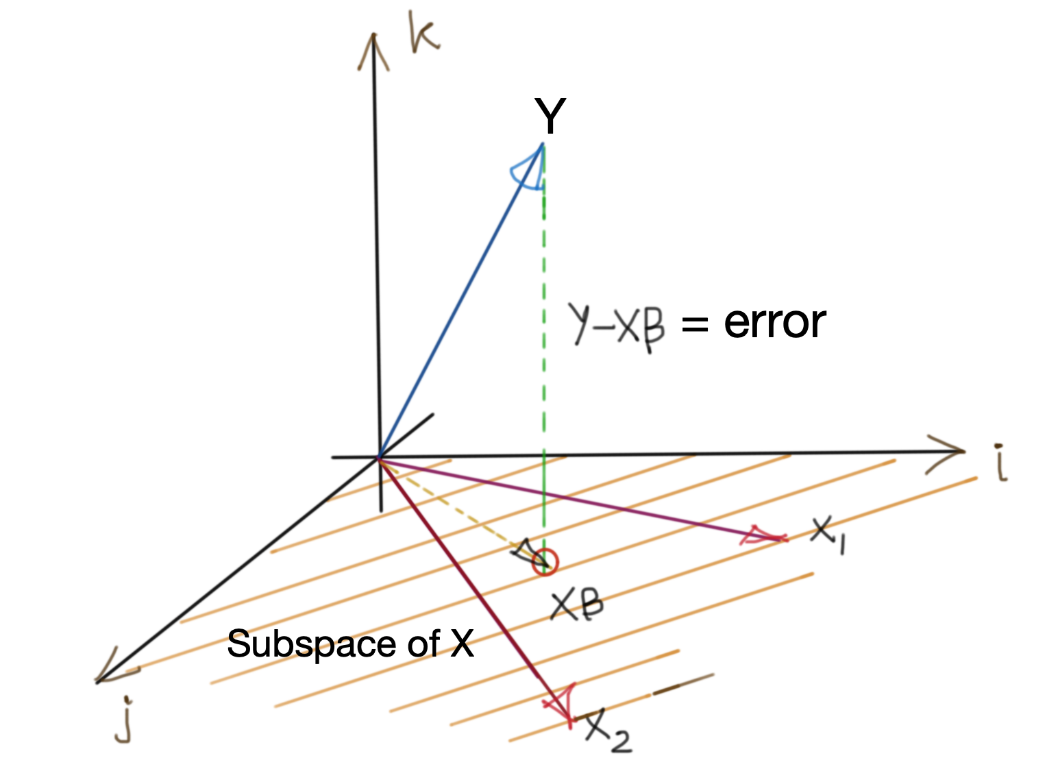
This implies that that the error vector \(Y-X\beta\) should be orthogonal to any vector in \(C(X\beta)\).

\[\langle X,Y-X\beta\rangle=0 \\ X^T(Y-X\beta)=0 \\ X^T(Y-X\beta)=0 \\ X^TY-X^TX\beta=0 \\ X^TX\beta=X^TY\]

Multiplying both sides by \({(X^TX)}^{-1}\) like we did earlier, we get:

\[{(X^TX)}^{-1}(X^TX)\beta={(X^TX)}^{-1}X^TY \\ \mathbf{\beta={(X^TX)}^{-1}X^TY}\]

which is the same result that we got in the previous section.

Footnotes

• Much of the intuition is from the books listed under References. If you have ever wondered: “How is the formula for the F-Test derived?”, or “Why do we use \(n-1\) in the denominator for sample variance instead of \(n\) without seeing Bessel’s Correction in every explanation?” I’d urge you to take a deeper look at these books.
• The F-statistic can also be derived using the above geometric intuitions; we will cover that in an upcoming post.

References:

• The Geometry of Multivariate Statistics : Thomas D. Wickens
• Statistical Methods: The Geometric Approach : David J. Saville, Graham R. Wood

---