The No-Questions Asked Guide to PyTorch : Part 1

Avishek Sen Gupta on 27 November 2022

Programming guides are probably the first posts to become obsolete, as APIs are updated. Regardless, we will look at building simple neural networks in PyTorch. We won’t be starting from models with a million parameters, however. We will proceed from the basics, starting with a single neuron, talk a little about the tensor notation and how that relates to our usual mathematical notation of representing everything with column vectors, and scale up from there.

I call this the “No Questions Asked” Guide, because I’d like to cut through all the diversions when learning a new API, and focus on communicating the basic ideas needed to get work done. Do I want to know how to set up a single neuron network? Yes. Am I interested in knowing why I call optimiser.zero_grad() before each training iteration? Maybe, but not immediately. If there are specific details I want to bring out later on, I will gladly modify these guides.

We will assume you have already installed Python and PyTorch; we’ll not get into those details. The progression for this post will be as follows:

One Neuron, One Input, No Bias, No Activation Function
One Neuron, One Input, No Bias, ReLU Activation Function
One Neuron, One Input, No Bias, Leaky ReLU Activation Function
One Neuron, One Input with Bias, Leaky ReLU Activation Function
One Neuron, Multiple Inputs with Bias, Leaky ReLU Activation Function
Multiple Neurons, Multiple Inputs with Bias, Leaky ReLU Activation Function
Multiple Neurons, One Hidden Layer, Multiple Inputs with Bias, Leaky ReLU Activation Function

Each of these build atop the previous one, with incremental changes.

1. One Neuron, One Input, No Bias, No Activation Function

This is the simplest setup one can imagine. We’ve stripped away every possible piece we could: the resulting thing is a neuron – barely. At this point, we are literally solving a multiplication problem: it could not get any simpler.

The architecture we are aiming for is like so:

One Neuron, One Input, No Bias, No Activation Function

import torch
import torch.nn as nn

class SimpleNN(nn.Module):
    def __init__(self):
        super(SimpleNN, self).__init__()
        self.first_layer = nn.Linear(1, 1, bias=False)

    def forward(self, x):
        return self.first_layer(x)


net = SimpleNN()
print(net)
print(list(net.parameters()))

learning_rate = 0.1
simple_optimiser = torch.optim.SGD(net.parameters(), lr = learning_rate, momentum=0.9)
target =torch.tensor([5.])
loss_criterion =nn.MSELoss()
net.train()

for i in range(100):
    simple_optimiser.zero_grad()
    output = net(torch.tensor([1.]))

    loss = loss_criterion(output, target)
    print(f"Loss = {loss}")

    loss.backward()
    simple_optimiser.step()

print(list(net.parameters()))
net.eval()
print(net(torch.tensor([1.])))

Let’s talk quickly about a couple of things.

The input is given as a tensor, and visually, it looks like a row vector. In our usual notation when dealing with linear functions, we use \(w^T x=C\), where \(w\) and \(x\) are column vectors. You can get the same result, just transposed, if you write \(x^T w = C^T\), which is the form that you get using PyTorch (since \(x^T\) is a row vector). \(C\) is a \(1 \times 1\) matrix, so the transpose doesn’t matter.
Printing out the network parameters (there is only one) gives us the sole weight as being very close to 5. This makes sense, since the only input we are training with is 1, and the target output is 5, thus the ideal weight value should be \(5/1=5\).
The error metric we are using is the Mean Squared Error.
The optimiser chosen is the Stochastic Gradient Descent algorithm; we may have more to say about it in an Optimisation series.

2. One Neuron, One Input, No Bias, ReLU Activation Function

Let’s add an activation function to the above example. This will be a Rectified Linear Unit (ReLU). The architecture we are aiming for is like so:

One Neuron, One Input, No Bias, ReLU

import torch
import torch.nn.functional as F
import torch.nn as nn

class SimpleNN(nn.Module):
    def __init__(self):
        super(SimpleNN, self).__init__()
        self.first_layer = nn.Linear(1, 1, bias=False)

    def forward(self, x):
        return F.relu(self.first_layer(x))


net = SimpleNN()
print(net)
print(list(net.parameters()))

learning_rate = 0.1
simple_optimiser = torch.optim.SGD(net.parameters(), lr = learning_rate, momentum=0.9)
target =torch.tensor([5.])
loss_criterion =nn.MSELoss()

net.train()

for i in range(100):
    simple_optimiser.zero_grad()
    output = net(torch.tensor([1.]))

    loss = loss_criterion(output, target)
    print(f"Loss = {loss}")

    loss.backward()
    simple_optimiser.step()

print(list(net.parameters()))
net.eval()
print(net(torch.tensor([1., 1.])))

If you run the above code a few times, you will find that, in some runs, there are no updates to the weights at all. The loss essentially stays constant. This is because the output of the neuron is less than zero, which clamps the output to zero, and thus kills the gradient in the backpropagation process. We will talk about this in a specific post on backpropagation.

3. One Neuron, One Input, No Bias, Leaky ReLU Activation Function

To rectify the above situation, we will use what is called the Leaky ReLU. This adds a small, but nonzero, gradient to the original ReLU function if the input is less than zero. This is demonstrated below:

import torch
import torch.nn.functional as F
import torch.nn as nn

class SimpleNN(nn.Module):
    def __init__(self):
        super(SimpleNN, self).__init__()
        self.first_layer = nn.Linear(1, 1, bias=False)

    def forward(self, x):
        return F.leaky_relu(self.first_layer(x))


net = SimpleNN()
print(net)
print(list(net.parameters()))
net.train()

learning_rate = 0.1
simple_optimiser = torch.optim.SGD(net.parameters(), lr = learning_rate, momentum=0.9)
target =torch.tensor([5.])
loss_criterion =nn.MSELoss()

for i in range(100):
    simple_optimiser.zero_grad()
    output = net(torch.tensor([1.]))

    loss = loss_criterion(output, target)
    print(f"Loss = {loss}")

    loss.backward()
    simple_optimiser.step()

print(list(net.parameters()))
net.eval()
print(net(torch.tensor([1., 1.])))

The architecture we’ll get is like so:

One Neuron, One Input, No Bias, Leaky ReLU

4. One Neuron, One Input with Bias, Leaky ReLU Activation Function

We now add the bias input to the neuron. This is as simple as setting bias=True in the above code, so that we get the following:

import torch
import torch.nn.functional as F
import torch.nn as nn

class SimpleNN(nn.Module):
    def __init__(self):
        super(SimpleNN, self).__init__()
        self.first_layer = nn.Linear(1, 1, bias=True)

    def forward(self, x):
        return F.leaky_relu(self.first_layer(x))


net = SimpleNN()
print(net)
print(list(net.parameters()))
net.train()

learning_rate = 0.1
simple_optimiser = torch.optim.SGD(net.parameters(), lr = learning_rate, momentum=0.9)
target =torch.tensor([5.])
loss_criterion =nn.MSELoss()

for i in range(100):
    simple_optimiser.zero_grad()
    output = net(torch.tensor([1.]))

    loss = loss_criterion(output, target)
    print(f"Loss = {loss}")

    loss.backward()
    simple_optimiser.step()

print(list(net.parameters()))
net.eval()
print(net(torch.tensor([1., 1.])))

The architecture we are aiming for is like so:

One Neuron, One Input with Bias, Leaky ReLU

5. One Neuron, Multiple Inputs with Bias, Leaky ReLU Activation Function

We will finally add another input to our neuron. This will complete our prototypical single perceptron model that we all know and love. The architecture we are aiming for is like so:

One Neuron, Multiple Inputs with Bias, Leaky ReLU

import torch
import torch.nn.functional as F
import torch.nn as nn

class SimpleNN(nn.Module):
    def __init__(self):
        super(SimpleNN, self).__init__()
        self.first_layer = nn.Linear(2, 1, bias=True)

    def forward(self, x):
        return F.leaky_relu(self.first_layer(x))


net = SimpleNN()
print(net)
print(list(net.parameters()))

learning_rate = 0.1
simple_optimiser = torch.optim.SGD(net.parameters(), lr = learning_rate, momentum=0.9)
target =torch.tensor([5.])
loss_criterion =nn.MSELoss()

for i in range(100):
    simple_optimiser.zero_grad()
    output = net(torch.tensor([1., 1.]))

    loss = loss_criterion(output, target)
    print(f"Loss = {loss}")

    loss.backward()
    simple_optimiser.step()

print(list(net.parameters()))
print(net(torch.tensor([1., 1.])))

6. Multiple Neurons, Multiple Inputs with Bias, Leaky ReLU Activation Function

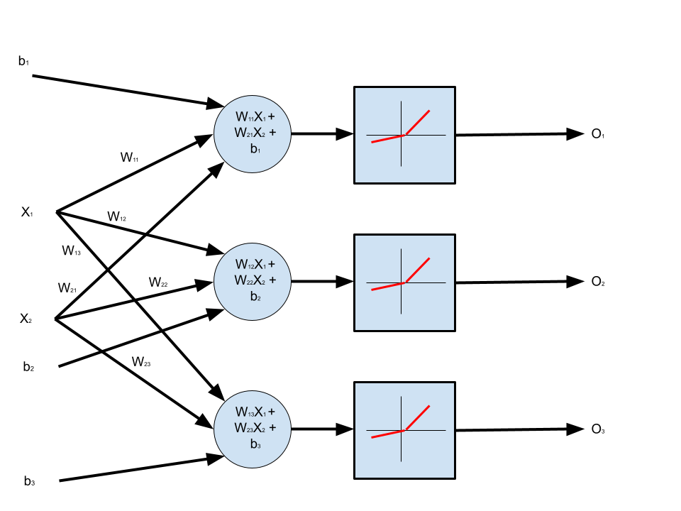
Now let’s talk of layers. We already have a single layer, but let’s add more than one neuron to this layer. Then, the architecture will look like the following:

Multiple Neurons, Multiple Inputs with Bias, Leaky ReLU

import torch
import torch.nn.functional as F
import torch.nn as nn

class SimpleNN(nn.Module):
    def __init__(self):
        super(SimpleNN, self).__init__()
        self.first_layer = nn.Linear(2, 3, bias=True)

    def forward(self, x):
        return F.leaky_relu(self.first_layer(x))


net = SimpleNN()
print(net)
print(list(net.parameters()))
net.train()

learning_rate = 0.1
simple_optimiser = torch.optim.SGD(net.parameters(), lr = learning_rate, momentum=0.9)
target =torch.tensor([5., 6., 7.])
loss_criterion =nn.MSELoss()

for i in range(100):
    simple_optimiser.zero_grad()
    output = net(torch.tensor([1., 1.]))

    loss = loss_criterion(output, target)
    print(f"Loss = {loss}")

    loss.backward()
    simple_optimiser.step()

print(list(net.parameters()))
net.eval()
print(net(torch.tensor([1., 1.])))
print(F.leaky_relu(torch.tensor([-1., 5.])))

Each neuron will still have its own individual output, rectified by a ReLU. A quirk (convenience?) of the ReLU class in PyTorch is that it takes a tensor and applies the rectification per-element. Thus, it really behaves as if there were \(n\) single element ReLUs, each connected to a single neuron, having its own output.

If we want to integrate all the outputs from a previous layer, we will need to add a new layer of neurons.

Another point to note is that the target tensor can either have a single value, in which case the network will be trained to output that single value on all its outputs, or the target tensor must have element-wise target outputs matching the number of outputs of the network.

The numbers in the constructor of the Linear class are worth reiterating about. The first parameter is the dimensionality of the input, i.e., Linear(2,3) implies that the input will be a two-dimensional tensor. The second parameter describes how many neurons (and consequently, how many outputs from this layer) this input will be fed to. Thus, Linear(2,3) implies that a two-dimensional tensor will be fed to 3 neurons.

7. Multiple Neurons, One Hidden Layer, Multiple Inputs with Bias, Leaky ReLU Activation Function

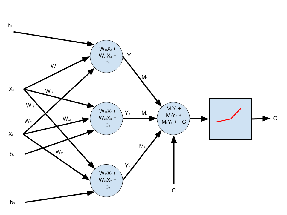
The architecture we are aiming for is that of a simple MultiLayer Perceptron (MLP), like so:

Multiple Neurons, Multiple Inputs with Hidden Layer and Bias, Leaky ReLU

import torch
import torch.nn.functional as F
import torch.nn as nn


class SimpleNN(nn.Module):
    def __init__(self):
        super(SimpleNN, self).__init__()
        self.first_layer = nn.Linear(2, 3, bias=True)
        self.second_layer = nn.Linear(3, 1, bias=True)

    def forward(self, x):
        return F.leaky_relu(self.second_layer(self.first_layer(x)))


net = SimpleNN()
print(net)
print(list(net.parameters()))
net.train()

learning_rate = 0.01
simple_optimiser = torch.optim.SGD(net.parameters(), lr=learning_rate, momentum=0.9)
target = torch.tensor([10.])
loss_criterion = nn.MSELoss()

for i in range(100):
    simple_optimiser.zero_grad()
    output = net(torch.tensor([1., 1.]))

    loss = loss_criterion(output, target)
    print(f"Loss = {loss}")

    loss.backward()
    for param in net.parameters():
        print(f"Param before ={param.grad}")
    simple_optimiser.step()
    for param in net.parameters():
        print(f"Param after ={param.grad}")

print(list(net.parameters()))
net.eval()
print(net(torch.tensor([1., 1.])))

We can refactor the network architecture to be more declarative. We do this by wrapping up all the layers into a Sequential pipeline, and simply invoking that pipeline in the forward() method.

import torch
import torch.nn.functional as F
import torch.nn as nn


class SimpleNN(nn.Module):
    def __init__(self):
        super(SimpleNN, self).__init__()
        self.stack = nn.Sequential(nn.Linear(2, 3, bias=True), nn.Linear(3, 1, bias=True), nn.LeakyReLU())

    def forward(self, x):
        return self.stack(x)


net = SimpleNN()
print(net)
print(list(net.parameters()))
net.train()

learning_rate = 0.01
simple_optimiser = torch.optim.SGD(net.parameters(), lr=learning_rate, momentum=0.9)
target = torch.tensor([10.])
loss_criterion = nn.MSELoss()

for i in range(100):
    simple_optimiser.zero_grad()
    output = net(torch.tensor([1., 1.]))

    loss = loss_criterion(output, target)
    print(f"Loss = {loss}")

    loss.backward()
    simple_optimiser.step()

print(list(net.parameters()))
print("Param Groups")
print(simple_optimiser.param_groups)
net.eval()
print(net(torch.tensor([1., 1.])))

tags: Machine Learning - PyTorch - Programming - Neural Networks

Total Internal Reflection

Code

Contact