Building a simple Virtual Machine in Prolog

Avishek Sen Gupta on 3 July 2025

In this post, I’ll talk about how I wrote a small Virtual Machine in Prolog which can both interpret concrete assembly language-like programs, and run basic symbolic executions, which are useful in data flow analyses of programs. The full code is available in this repository.

This post has not been written or edited by AI.

Building a simple Virtual Machine

One of my favourite exercises to do when learning a new language is to build something which exercises non-trivial capabilities of the language like pattern matching, flexibility of data structures, or exposes the brevity of expressing ideas in the langauge. Building a simple virtual machine forces one to reckon with ideas like expression trees, recursive traversals, term rewriting, etc.

I’ve also been reading about symbolic execution as a way to perform dataflow analysis recently as well. As an added challenge, I chose to enhance the concrete interpretation of a program with symbolic execution capabilities.

Foundational Operations from the ground-up

We need a dictionary implementation. SWI-Prolog has the dictionaries, but since we are building everything from scratch, we will write a very naive implementation using only lists. Granted, there are some semantics of a dictionary that can be violated for now - for example, you can start off with duplicate keys, but let’s assume the happy path.

get2(_,[],empty).
get2(K, [(-(K,VX))|_],VX) :- !.
get2(K, [_|T],R) :- get2(K,T,R).

put2_(-(K,V),[],Replaced,R) :- Replaced->R=[];R=[-(K,V)].
put2_(-(K,V),[-(K,_)|T],_,[-(K,V)|RX]) :- put2_(-(K,V),T,true,RX).
put2_(-(K,V),[H|T],Replaced,[H|RX]) :- put2_(-(K,V),T,Replaced,RX).

put2(-(K,V),Map,R) :- put2_(-(K,V),Map,false,R).

To represent entries in a dictionary, we use the K-V compound term, which is basically syntactic sugar for -(K,V). These entries live inside a list. Both get2 and put2 behave in predictable ways, except when the dictionary has duplicate keys. In that case:

get2(K,V) returns the value of the first matching key.
put2(-(K,V),InputMap,OutputMap) modifies all matching keys with the value V.

In our current implementation, we will not worry about duplicate entries yet.

We will also need push/pop operations on stacks. This is very simple. Note that the top of the stack is always the leftmost element.

push_(V,Stack,UpdatedStack) :- UpdatedStack=[V|Stack].
pop_([],empty,[]).
pop_([H|Rest],H,Rest).

Logging

We will be logging quite a bit inside the rules. Thus it is important to have a structured way of logging different levels, like DEBUG, INFO, WARNING, etc. This is what a basic logging setup looks like:

log_with_level(LogLevel,FormatString,Args) :- format(string(Message),FormatString,Args),format('[~w]: ~w~n',[LogLevel,Message]).

debug(Message) :- log_with_level('DEBUG',Message,[]).
debug(FormatString,Args) :- log_with_level('DEBUG',FormatString,Args).

info(Message) :- log_with_level('INFO',Message,[]).
info(FormatString,Args) :- log_with_level('INFO',FormatString,Args).

warning(Message) :- log_with_level('WARN',Message,[]).
warning(FormatString,Args) :- log_with_level('WARN',FormatString,Args).

error(Message) :- log_with_level('ERROR',Message,[]).
error(FormatString,Args) :- log_with_level('ERROR',FormatString,Args).

dont_log(_).
dont_log(_,_).

Minimal instruction set

The minimal instruction is comprised of the following:

mov(reg,reg|constant)
cmp(reg,reg|constant)
label(name)
j(label)
jz(label|address)
jnz(label|address)
push(reg|constant)
pop(reg)
call(label)
ret
hlt
term(string)
nop
inc(reg)
dec(reg)
mul(reg,reg|constant)
term(string)

Registers, Flags, and other Data Structures

For convenience, I chose to not have a fixed number of registers for convenience; thus, you can use any symbol as a register. In this respect, we will be treating registers more akin to conventional variables.

There will be one special register called the Instruction Pointer (IP). This will point to the next instruction to be executed. Jump instructions like j, jnz, and jz can can modify the IP to change the flow of the program.

The other useful data structure will be the stack, which is operated by push, pop, call, and ret (the last two use it to keep track of the stack when entering and leaving procedures).

There will be one flag called the Zero Flag. This should probably be better named to Equals Flag, because it is set to zero if the two sides of a cmp are equal, otherwise -1/+1 depending upon their relative ordering.

Data can be of two types:

Concrete data, like numbers, which would be represented like const(5)
Symbolic data, which stand in for concrete data, and are used for symbolic execuction, which we’ll introduce in Symbolic Execution and World Splits. These are represented as sym(x), sym(abcd), etc.

Memory Model

For the purposes of this simple VM, I chose not to have any memory. I may add it later, and then I will update this post accordingly.

Execution Model

The execution model is simple and similar to what we’d expect a very simple single-threaded VM to behave. Every instruction is sequentially mapped to a specific memory address (simple incrementing integers for our purposes). The Instruction Pointer starts at 0. At every instruction, something can happen. Actions include:

Moving data between registers
Loading constants into registers
Incrementing / Decrementing registers
Push / pop values to / from the stack
Unconditional / Conditional jumps to another address
Compare registers to other registers or constants
Halt (effectively exit the program)
Declare a label
Call and return from a procedure (defined as a label)

Jumps work by modifying the value of the Instruction Pointer to the destination address. Procedure calls work similarly, but with an added side effect: the address of the instruction after the call is pushed onto the stack: when a ret is encountered, the topmost value is popped off the stack and is assigned back to the Instruction Pointer. This simulates the return from the procedure.

There are a couple of mappings we need to build to be able to jump to arbitrary locations because of changes to the IP.

Mapping labels to memory addresses
Mapping memory addresses to instructions

These mappings are done in the following code:

instruction_pointer_map([],IPMap,_,IPMap).
instruction_pointer_map([Instr|T],IPMap,IPCounter,FinalIPMap) :- put2(-(IPCounter,Instr),IPMap,UpdatedIPMap),
                                                                 plusOne(IPCounter,UpdatedIPCounter),
                                                                 instruction_pointer_map(T,UpdatedIPMap,UpdatedIPCounter,FinalIPMap).
label_map([],LabelMap,_,LabelMap).
label_map([label(Label)|T],LabelMap,IPCounter,FinalLabelMap) :- put2(-(label(Label),IPCounter),LabelMap,UpdatedLabelMap),
                                                                 plusOne(IPCounter,UpdatedIPCounter),
                                                                 label_map(T,UpdatedLabelMap,UpdatedIPCounter,FinalLabelMap),
                                                                 !.
label_map([_|T],LabelMap,IPCounter,FinalLabelMap) :- plusOne(IPCounter,UpdatedIPCounter),
                                                     label_map(T,LabelMap,UpdatedIPCounter,FinalLabelMap).

The label_map predicate simply step through the full list of instructions, adding a label mapping to the current address (incremented each time through plusOne) when it encounters a label fact.

The instruction_map predicate simply assigns every instruction that it finds to an incrementing counter.

Symbolic Execution and World Splits

Symbolic execution is a technique used to determine the provenance of data in a piece of code. Assume, you have a very simplified code segment, like so:

Code=[
    mvc(reg(hl),const(10)), % load 10 into register HL
    mvc(reg(bc),const(5)),  % load 5 into register BC
    inc(reg(hl)),           % increment HL by one
    mul(reg(hl),reg(bc))    % multiply contents of HL with that of BC, store the result in HL
].

Now, suppose you wished to determine what sort of data transformations were taking place in this code. You might want to do this for different reasons:

Determine if there are any optimisations that can be made, eg: an addition of zero can be eliminated, since it does not change the answer.
Understand the data transformation for reverse engineering the business logic of this code

Now, you can run this piece of code on concrete numbers and generate lots of test cases for different values in hl, bc, etc. However, as a human, you may be able to induce a generic rule which explains the behaviour of this piece of code, which is:

hl=(hl+1)*bc

To deduce this rule, note that you didn’t use a concrete number, you used symbols like hl and bc to represent the values that these registers could store. Symbolic execution does exactly this: instead of storing concrete numbers in registers, we store symbols. When we “execute” the program, all operations which modify these symbols essentially store the log of operations on these symbols. So for example:

Code=[
mvc(reg(hl),sym(a)), % load symbol a into register HL
mvc(reg(bc),sym(b)),  % load symbol b into register BC
inc(reg(hl)),           % increment HL by one, HL now holds inc(sym(a))
mul(reg(hl),reg(bc))    %  HL now holds mul(inc(sym(a)),sym(b))
].

Thus at the end hl’s contents are mul(inc(sym(a)),sym(b)), which is interpreted as hl=(hl+1)*bc.

Symbolic execution is a powerful technique for program analysis. There is however one wrinkle we need to take care of when building a symbolic interpreter: branching.

Consider the instruction jz(label(some_label)). During concrete execution, we can look at the value of the Zero Flag, and then determine whether we want to jump to some_label or continue with the normal execution flow. However, the Zero Flag is set based on comparison between two concrete values: what if those values are symbols? You cannot meaningfully compare sym(a) and sym(b) numerically: they represent a range of values.

So, then the question becomes: which path do we take?

The image below is an example of the sort of situation you might encounter at a branch point.

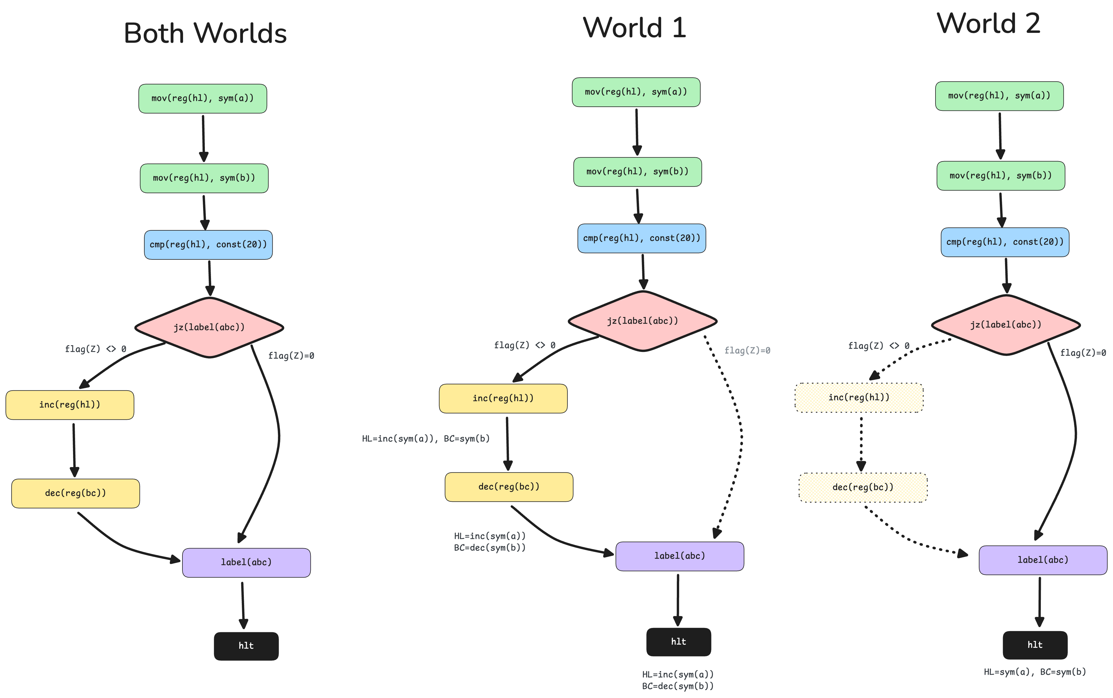
Symbolic Execution World Splitting

The answer is that we take both paths. Effectively, we split our execution world into two branches: one which makes the jump, and the other one which contains normal execution. These two branches then continue on as individual threads to completion. Of course, if these branches encounter more conditional jump instructions, more sub-worlds split out of these as well, and so on.

Symbolic execution thus explores all possibilities of a program.

One issue is that this can easily result in a combinatorial explosion of paths, as each binary branch doubles the number of effective worlds. Symbolic execution engines tackle this in various ways. However, for our simple VM, we will simply keep splitting our world into new branches whenever we encounter conditional jumps.

Arithmetic operations

plusOne(sym(X),sym(inc(sym(X)))).
plusOne(const(X),const(PlusOne)) :- PlusOne is X+1.

minusOne(sym(X),sym(dec(sym(X)))).
minusOne(const(X),const(MinusOne)) :- MinusOne is X-1.

product(const(LHS),const(RHS),const(Product)) :- Product is LHS*RHS.
product(sym(LHS),sym(RHS),sym(product(sym(LHS),sym(RHS)))).
product(sym(LHS),const(RHS),sym(product(sym(LHS),const(RHS)))).
product(const(LHS),sym(RHS),sym(product(const(LHS),sym(RHS)))).

The predicate definitions take into account meaningful combinations of constants and symbols. As a rule of thumb, any expression containing even one symbol cannot be simplified (save degenerate cases like adding / subtracting 0, multiplying by 1 or 0, subtracting an expression from itself, etc., but we leave those aside for now for simplicity). Thus the only arithmetic simplification we do is when everything in an expression is a constant. For all the others, it creates a new compound term which reflects the operation being performed, which will ultimately be inspected at the end of a run as part of the value of a register.

Comparison

Comparison also works similar to arithmetic operations, in that actual comparison is usually only performed when both sides are constants. The special case is that if both sides are symbolic expressions with the same structure, that also counts for equality. Otherwise a new compound term logging the comparison operator (wrapped in a symbol itself) is returned.

equate(LHS,LHS,const(0)).
equate(sym(LHS),sym(RHS),sym(cmp(sym(LHS)),sym(RHS))).
equate(sym(LHS),const(RHS),sym(cmp(sym(LHS)),const(RHS))).
equate(const(LHS),sym(RHS),sym(cmp(const(LHS)),sym(RHS))).
equate(const(LHS),const(RHS),const(1)) :- LHS < RHS.
equate(const(LHS),const(RHS),const(-1)) :- LHS > RHS.

Virtual Machine state

The virtual machine state must reflect the exact configuration of registers, flags, stack, etc. These are represented as:

vmState(IP,Stack,CallStack,Registers,flags(zero(v1),hlt(v2),branch(v3))

IP: Instruction Pointer, represented as a const()
Stack: The program writer’s stack
CallStack: We need a stack to store return addresses when performing procedure calls. However, using the program writer’s stack would mess with expectations of the programmer of what should be at the top of the stack. Therefore, a separate call stack is maintained.
Registers: A map of the registers with their values
Flags: The only flag that a user can set and access (indirectly) is the Zero Flag. However, there are two other (hidden flags) which indicate whether the program is about to halt or branch. The branch() compound term is useful to keep track of when to split worlds during symbolic execution. The hlt() compound term is to keep track of a halt condition (which can be an explicit HLT instruction, or the flow falling off the end of a program without a HLT instruction).

This vmState compound term is passed around everywhere and essentially is equivalent to a struct in C (SWI-Prolog has dedicated facilities for representing structures, but I’ve deliberately kept the code as implementation-neutral as possible).

Accessing data inside this structure is very easy, thanks to unification and pattern matching; for example, if we wished to only extract the value of the Zero Flag, and not care about the other values, we can simply write:

vmState(_,_,_,_,flags(zero(ZeroFlagValue),_,_)

Inner single world loop

For reference, this is the high level predicate flow that we will be referencing in the explanation of the predicates.

Symbolic Interpreter Flow

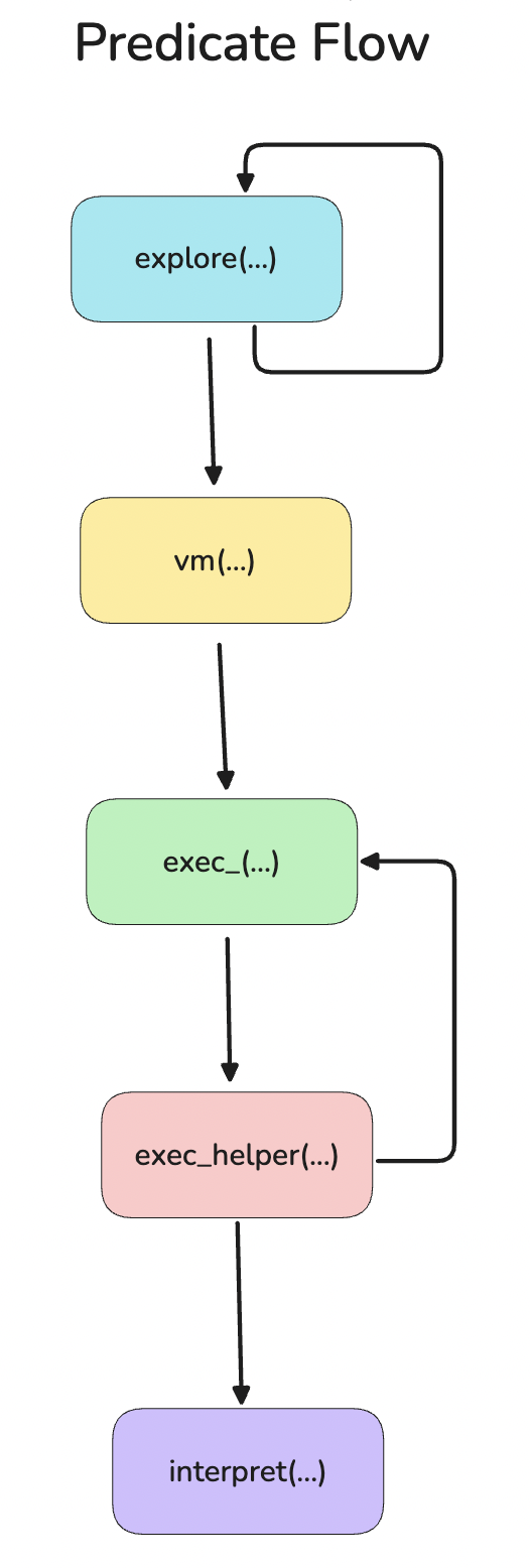
Before looking at how branches in symbolic execution are handled, it is instructive to understand how a single world, concrete execution flow works. The inner loop which evaluates a world, starts with:

The original program, which simply a list of instructions
The ExecutionMode is either symbolic or concrete. For the purposes of this explanation, let us assume that it is concrete.
The StateIn is simply the initial VM state which is described in Virtual Machine state
The vmMaps is a tuple of the IP Map and the label map, as described in Building the navigation maps
The last variable represents the final output of evaluating this particular world. In particular, the TraceOut contains the program trace for this execution. Since we are only doing a concrete flow, there will be no ChildWorlds. The code below represents the part of the vm predicate which is pertinent to this discussion.

vm(Program,ExecutionMode,StateIn,vmMaps(IPMap,LabelMap),world(StateIn,TraceOut,ChildWorlds)) :-
                              exec_(vmMaps(IPMap,LabelMap),
                                  StateIn,[],
                                  traceOut(FinalTrace,VmStateOut),
                                  env(log(debug,info,warning,error),ExecutionMode)),
                              VmStateOut=vmState(FinalIP,FinalStack,FinalCallStack,FinalRegisters,FinalVmFlags),
                              minusOne(FinalIP,LastInstrIP),
                              TraceOut=traceOut(FinalTrace,vmState(LastInstrIP,FinalStack,FinalCallStack,FinalRegisters,FinalVmFlags)),
                              ...
                              .

The core interpretation is triggered by the exec_ predicate. The remaining lines involves taking the output VM state, adjusting its final IP value (which is one address beyond the last executed instruction) to point to the last executed instruction, and repackaging it to bind it to the output variable TraceOut.

Let’s look at the internal exec_ loop. The exec_ has two cases:

The base case is if the hlt flag is set to true (hlt(true)). This indicates that a HLT instruction has been encountered in the execution of the previous instruction. At this point, the TraceOut variable is bound to the accumulated program trace and the current VM trace, and returned back to the vm_ predicate.

exec_(_,vmState(IP,Stack,CallStack,Registers,flags(ZeroFlag,hlt(true),BranchFlag)),
                  TraceAcc,
                  traceOut(TraceAcc,vmState(IP,Stack,CallStack,Registers,flags(ZeroFlag,hlt(true),BranchFlag))),
                  env(log(_,Info,_,_),_)) :- call(Info,'EXITING PROGRAM LOOP!!!').

For the general case (when the last instruction was not HLT), we first get the instruction corresponding to the current IP value from the IPMap structure. This is then passed to exec_helper with all the associated context.

exec_(vmMaps(IPMap,LabelMap),vmState(IP,Stack,CallStack,Registers,VmFlags),TraceAcc,StateOut,Env) :-
                                                    get2(IP,IPMap,Instr),
                                                    exec_helper(Instr,vmMaps(IPMap,LabelMap),
                                                        vmState(IP,Stack,CallStack,Registers,VmFlags),TraceAcc,StateOut,Env).

The exec_helper predicate is where the interpretation actually happens. This also has two cases.

The base case is when an empty instruction is encountered. This can happen if the program does not contain a HLT instruction, and execution falls off the end of the program. This is treated equivalent to an implicit HLT instruction. Thus, the TraceOut variable is bound to whatever context is already present. The only explicit modification is the hlt flag which is explicitly set to true.

exec_helper(empty,VmMaps,vmState(IP,Stack,CallStack,Registers,flags(ZeroFlag,_,BranchFlag)),
                    TraceAcc,
                    traceOut(TraceAcc,ExitState),
                    env(log(Debug,Info,Warn,Error),ExecutionMode)) :-
                            ExitState=vmState(IP,Stack,CallStack,Registers,flags(ZeroFlag,hlt(true),BranchFlag)),
                            call(Warn,'No other instruction found, but no HLT is present. Halting program.'),
                            exec_(VmMaps,ExitState,TraceAcc,traceOut(TraceAcc,ExitState),env(log(Debug,Info,Warn,Error),ExecutionMode)).

The general case is the actual interpretation of the instruction. Before the interpret predicate is called, a NextIP variable is initialised to the current IP incremented by one, to indicate the next instruction that will be executed, assuming there are no jumps. This is so that a conditional jump can either return the same NextIP (i.e., no jump), or can return a different IP (indicating a jump).

The interpret predicate is then called, which has different cases, depending upon the instruction encountered. The various cases are described in Instruction Interpretation.

The shouldBranch() ternary operator’s true condition is only triggered during symbolic execution, so we’ll not worry about that for the moment. The negative condition is the concrete execution flow. This part is straightforward. It simply calls the exec_ predicate recursively with the updated IP.

This mutual recursive call between exec_ and exec_helper continues until a halt condition is reached.

exec_helper(...) :-
        ...,
        plusOne(IP,NextIP),
        interpret(Instr,VmMaps,vmState(NextIP,Stack,CallStack,Registers,VmFlags),vmState(UpdatedIP,UpdatedStack,UpdatedCallStack,UpdatedRegisters,UpdatedVmFlags),env(log(Debug,Info,Warning,Error),ExecutionMode)),
        (shouldBranch(UpdatedVmFlags)->
            (
                ...
            );
            (
                call(Debug,'Next IP is ~w',[UpdatedIP]),
                exec_(VmMaps,vmState(UpdatedIP,UpdatedStack,UpdatedCallStack,UpdatedRegisters,UpdatedVmFlags),TraceAcc,traceOut(RemainingTrace,vmState(FinalIP,FinalStack,FinalCallStack,FinalRegisters,FinalVmFlags)),env(log(Debug,Info,Warning,Error),ExecutionMode)),
                FinalTrace=[traceEntry(Instr,vmState(UpdatedIP,UpdatedStack,UpdatedCallStack,UpdatedRegisters,UpdatedVmFlags))|RemainingTrace]
            )
        ),
        !.

Some notes on Instruction Interpretation

Many of the cases for the interpret predicate are about retrieving the values of (one or two) registers, performing some manipulation on them (symbolic or arithmetic) and storing the result in the register, as in this example for the MUL instruction.

interpret(mul(reg(LHSRegister),reg(RHSRegister)),_,vmState(NextIP,Stack,CallStack,Registers,VmFlags),vmState(NextIP,Stack,CallStack,UpdatedRegisters,VmFlags),env(log(Debug,_,_,_),_)) :-
                get2(LHSRegister,Registers,LHSValue),
                get2(RHSRegister,Registers,RHSValue),
                call(Debug,'LHS is ~w,~w',[LHSRegister,LHSValue]),
                call(Debug,'RHS is ~w,~w',[RHSRegister,RHSValue]),
                product(LHSValue,RHSValue,Product),
                call(Debug,'And result is ~w',[Product]),
                update_reg(-(reg(LHSRegister),Product),Registers,UpdatedRegisters).

The two get2 calls retrieve the values of LHSRegister and RHSRegister. product calculates their (symbolic or arithmetic) product. update_reg updates the LHSRegister with the product.

The two instructions that modify the VM state differently are the JZ and JNZ instructions, which we have discussed depend upon whether the ExecutionMode is symbolic or concrete.

Symbolic Execution and World splitting: The outer loop

Let’s talk about how symbolic execution works. The symbolic execution mode is controlled by two variables:

The ExecutionMode variable which can either be symbolic or concrete.
The branch flag which is explicitly set to true by conditional jump instructions, only when the ExecutionMode is symbolic. To see this link, look at the two cases for the JZ (Jump if Zero) instruction.

interpret(jz(JumpIP),_,vmState(OldNextIP,Stack,CallStack,Registers,VmFlags),vmState(UpdatedIP,Stack,CallStack,Registers,UpdatedVmFlags),env(_,mode(symbolic))) :- interpret_symbolic_condition(OldNextIP,JumpIP,VmFlags,isZero,UpdatedVmFlags,UpdatedIP).
interpret(jz(JumpIP),_,vmState(OldNextIP,Stack,CallStack,Registers,VmFlags),vmState(UpdatedIP,Stack,CallStack,Registers,UpdatedVmFlags),env(_,mode(concrete))) :- interpret_condition(OldNextIP,JumpIP,VmFlags,isZero,UpdatedVmFlags,UpdatedIP).

The first case triggers when the mode is symbolic, and calls the interpret_symbolic_condition predicate. This predicate is a single predicate which directly sets branch(true):

interpret_symbolic_condition(OldNextIP,_,flags(ZeroFlag,HltFlag,_),_,flags(ZeroFlag,HltFlag,branch(true)),OldNextIP).

The second case triggers when the mode is concrete and calls the interpret_condition predicate which is described in Instruction Interpretation.

Where is branch(true) actually used? This is in the exec_helper predicate, reproduced here with the pertinent code:

exec_helper(...) :-
    ...,
    (shouldBranch(UpdatedVmFlags)->
        (
            terminateForBranch(vmState(UpdatedIP,UpdatedStack,UpdatedCallStack,UpdatedRegisters,UpdatedVmFlags),vmState(FinalIP,FinalStack,FinalCallStack,FinalRegisters,FinalVmFlags)),
            FinalTrace=TraceAcc
        );
        (
            ...
        )
    ),
    !.

The shouldBranch() term is only true when branch(true) is true. At this point, it simply returns the entire trace and the VM state as-is, effectively ending the execution of this thread. This is because, beyond this, two new world threads need to be created and run interpreted as their own worlds with identical starting points.

Where does this world splitting take place? This happens in the vm() predicate, reproduced here with the relevant code

vm(...) :-
      ...,
      (shouldTerminateWorld(FinalVmFlags)->(...);
        (
          NewStartIP_One=FinalIP,
          branchDestination(LastInstrIP,LabelMap,IPMap,NewStartIP_Two),
          Branches=[NewStartIP_One,NewStartIP_Two],
          info("Branches are: ~w",[Branches]),
          explore(Program,ExecutionMode,VmStateOut,vmMaps(IPMap,LabelMap),Branches,[],ChildWorlds)
        )
      ).

At this point, we are back at the top, and we need to decide whether to halt the execution entirely, or whether to branch out into different worlds. How do we determine this?

Answer: We know we are back at the top, but we also know that we aren’t in a HALT condition (an explicit HALT instruction or execution flow falling off the end), therefore we must be at a branch point. Therefore, we extract two IP values, NewStartIP_One (the default execution flow IP value) and NewStartIP_Two (the jump IP value). Now, we recursively call the explore predicate, which is the top-level entry predicate for our VM.

Execution entry point

Let’s look at the explore predicate. The important variable in this predicate is the list of Instruction Pointers. If there is only one IP value (which is what happens when this predicate is first invoked), that means there is only one branch / world. If there are two (or more, though that is not a situation that happens with this VM), it means that there are multiple branches which need to be symbolically interpreted independently, starting from the same set of initial conditions (the VM state, etc.). explore is thus called recursively for every conditional branch, until there are none left, thus signalling the end of the symbolic execution tree.

explore(_,_,_,_,[],WorldAcc,WorldAcc).
explore(Program,ExecutionMode,VmState,VmMaps,[IP|OtherIPs],WorldAcc,[WorldOut|OtherWorldOuts]) :-
        VmState=vmState(_,Stack,CallStack,Registers,flags(ZeroFlag,_,_)),
        FreshState=vmState(IP,Stack,CallStack,Registers,flags(ZeroFlag,hlt(false),branch(false))),
        vm(Program,ExecutionMode,FreshState,VmMaps,WorldOut),
        explore(Program,ExecutionMode,VmState,VmMaps,OtherIPs,WorldAcc,OtherWorldOuts),
        !.

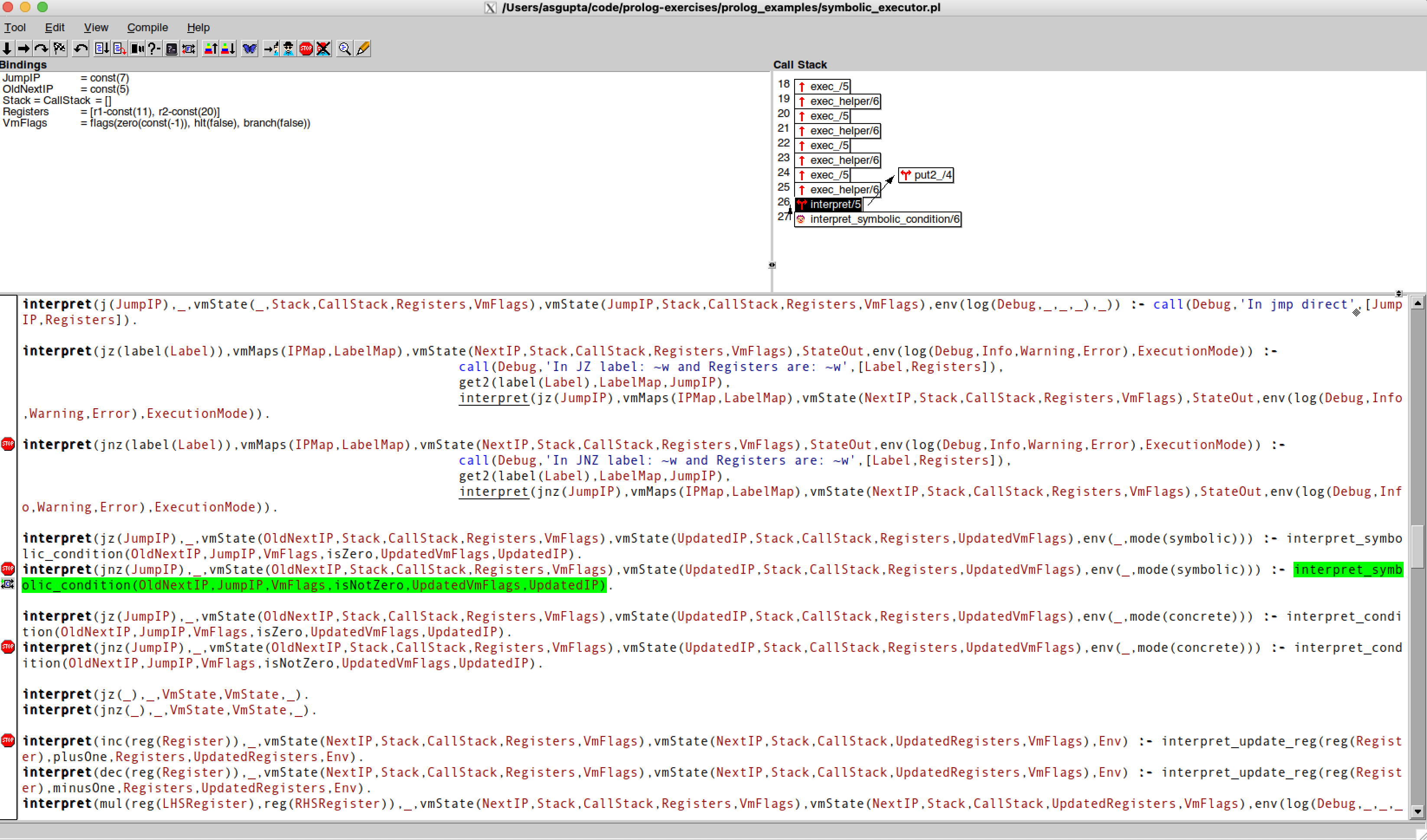
If you wish to trace the flow yourself and are using SWI-Prolog, I’d highly recommend using the graphical debugger. It has full support for breakpoints, step over/step into, forcing predicates to fail, on-the-fly edit-and-recompile, and more.

SWI-Prolog Graphical Debugger

Example Programs

These are a couple of example programs you can run with this VM.

Factorial

execute_symbolic([
     mov(reg(r0),const(5)),
     mov(reg(r1),const(1)),
     call(label(factorial)),
     push(const(30)),
     cmp(reg(r1),const(121)),
     hlt,
     label(factorial),
     cmp(reg(r0),const(0)),
     jz(label(base)),
     push(reg(r0)),
     dec(reg(r0)),
     call(label(factorial)),
     pop(reg(r0)),
     mul(reg(r1),reg(r0)),
     ret,

     label(base),
     mov(reg(r1),const(1)),
     ret
],
mode(concrete),AllWorlds),print_worlds(AllWorlds,0).

Symbolic execution example

execute_symbolic([
    mov(reg(r1),const(10)),inc(reg(r1)),
    mov(reg(r2),const(20)),
    cmp(reg(r1), const(0)),
    jnz(const(7)),
    cmp(reg(r2), const(1)),
    mov(reg(r1),const(30)),
    jz(const(10)),
    mov(reg(r3), const(40)),
    hlt,
    mov(reg(r3), const(50)),
    hlt
],
mode(symbolic),AllWorlds),print_worlds(AllWorlds,0).

Program statistics

The first observation I had about the code is that it is dense. There is minimal syntactic overhead, associated with imperative or object oriented programming. Unification ensures that there are no verbose assignment statements, no special syntax to pack and unpack structures. There are a couple of places assignment is used, but it is mostly to improve readability.
To get a sense of the expressiveness of the language due to its unification and pattern matching features, the original concrete interpreter (without the symbolic interpretation) was less than 50 lines of code.
The current version of the symbolic interpreter, excluding the data structures built from the ground up, takes up around 120 lines of code.

References

Symbolic Interpreter

tags: Prolog - Logic Programming - Virtual Machine - Symbolic Execution

Total Internal Reflection

Code

Contact