Vector Calculus: Graphs, Level Sets, and Constraint Manifolds

Avishek Sen Gupta on 20 April 2021

---

In this article, we take a detour to understand the mathematical intuition behind Constrained Optimisation, and more specifically the method of Lagrangian multipliers. We have been discussing Linear Algebra, specifically matrices, for quite a bit now. Optimisation theory, and Quadratic Optimisation as well, relies heavily on Vector Calculus for many of its results and proofs.

Most of the rules for single variable calculus translate over to vectors calculus, but now we are dealing with vector-valued functions and partial differentials.

This article will introduce the building blocks that we will need to reach our destination of understanding Lagrangians, with slightly more rigour than a couple of contour plots. Please note that this is in no way an exhaustive introduction to Vector Calculus, only the concepts necessary to progress towards the stated goal are introduced. If you’re interested in studying the topic further, there is a wealth of material to be found.

We will motivate most of the theory by illustrating the two-dimensional case in pictures, but understand that in actuality, we will often deal with higher-dimensional vector spaces.

Before we delve into the material proper, let’s look at the big picture approach that you will go through as part of this.

• Orthogonal Complements
• Graphs and Level Sets
• Gradients and Jacobians (We will not cover the basic material here too much, there may be other standalone posts about them, though)
• Tangent Spaces
• Parameterisation in an underdetermined system of Linear Equations

Required Review Material

• Matrix Intuitions
• Matrix Rank and Some Results
• Intuitions about the Orthogonality of Matrix Subspaces

Linear Algebra: Quick Recall and Some Identities

The reason we revisit this topic is because I want to introduce some new notation notation, and talk about a couple of properties you may or may not be aware of.

Orthogonal Complements

We have already met Orthogonal Complements in Intuitions about Matrix Subspaces, when we were talking about column spaces, row spaces, null spaces, and left null spaces. Recalling quickly, the column space and the left null space are mutually orthogonal complements, and the row space and the null space are mutually orthogonal complements.

The other fact worth recalling is that the column rank of a matrix is equal to its row rank. Since the rank of a matrix determines the dimensionality of a vector subspace (1 if it is a line, 2 if it’s a plane, and so on), it follows that the column space and row space of a matrix have the same dimensionality. Note that this dimensionality is not dependent on dimensionality of the vector space that the row/column space is embedded in, for example, a 1D subspace (a line) can exist in a three-dimensional vector space.

One (obvious) fact is that the dimensionality of the ambient vector space \(V\) is equal to or larger than the dimensionality of its row space/column space/null space/left null space of \(A\). That is:

\[dim(V)\geq dim(S) \| S\in {C(A), R(A), LN(A), N(A)}\]

We will make more precise statements about these relationships in the next section on Rank-Nullity Theorem.

Rank Nullity Theorem

The Rank Nullity Theorem states that the sum of the dimensionality of the column space (rank) and that of its orthogonal complement, left null space, (nullity) is equal to the dimension of the vector space they are embedded in. By the same token, the the dimensionality of the row space (rank) and that of its orthogonal complement, the null space, (nullity) is equal to the dimension of the vector space they are embedded in.

Mathematically, this implies:

\[\mathbf{dim(C(A))+dim(LN(A))=dim(V) \\ dim(R(A))+dim(N(A))=dim(V)}\]

where \(V\) is the embedding space. This always ends up as the number of basis vectors required to uniquely identify a vector in \(V\). To take a motivating example:

• A vector \(U=(1,2,3)\) requires three basis vectors (\((1,0,0), (0,1,0), (0,0,1)\)) to specify it completely in \({\mathbb{R}}^3\). Note that this is choice of basis vectors is not unique; I simply picked the standard basis vectors to illustrate the point. Thus \(dim(U)\) in this case is 3.
• The dimensionality of \(V=(1,2,3)\) is 1, since it is a vector. The column space of this “matrix” \(\begin{bmatrix} 1 \\ 2 \end{bmatrix}\) is basically a straight line extending infinitely long in both directions of this vector.
• To fully cover the ambient vector space \(V={\mathbb{R}}^3\), you need a vector space which is a plane, which is a two-dimensional subspace. This is mechanically deducible from the Rank-Nullity Theorem (3-1=2), but you can also intuit that the entire 3D space \(\mathbb{R}^n\) can be covered by taking a plane and translating it infinitely forwards and backwards along the vector \(U\).
• The plane we would like to pick is the orthogonal complement of \(V\), i.e., the plane \(P=x+2y+3z=0\). Can you see why it’s an orthogonal complement? Taking the dot product of any vector in the plane \(P\) (like \((-5,1,1)\)) and vector \(V\) gives us zero.
• It is also clear that to represent this plane in the form of a vector subspace (i.e., matrix form), we need two linearly independent 3D column vectors. This will automatically imply that the rank of this matrix is 2, which validates the conclusion that we drew earlier from the Rank-Nullity Theorem.

Subset containership of Orthogonal Complements

This rule is pretty simple, it states the following:

If \(U\subset V\), then \(U^{\perp}\supset V^{\perp}\)

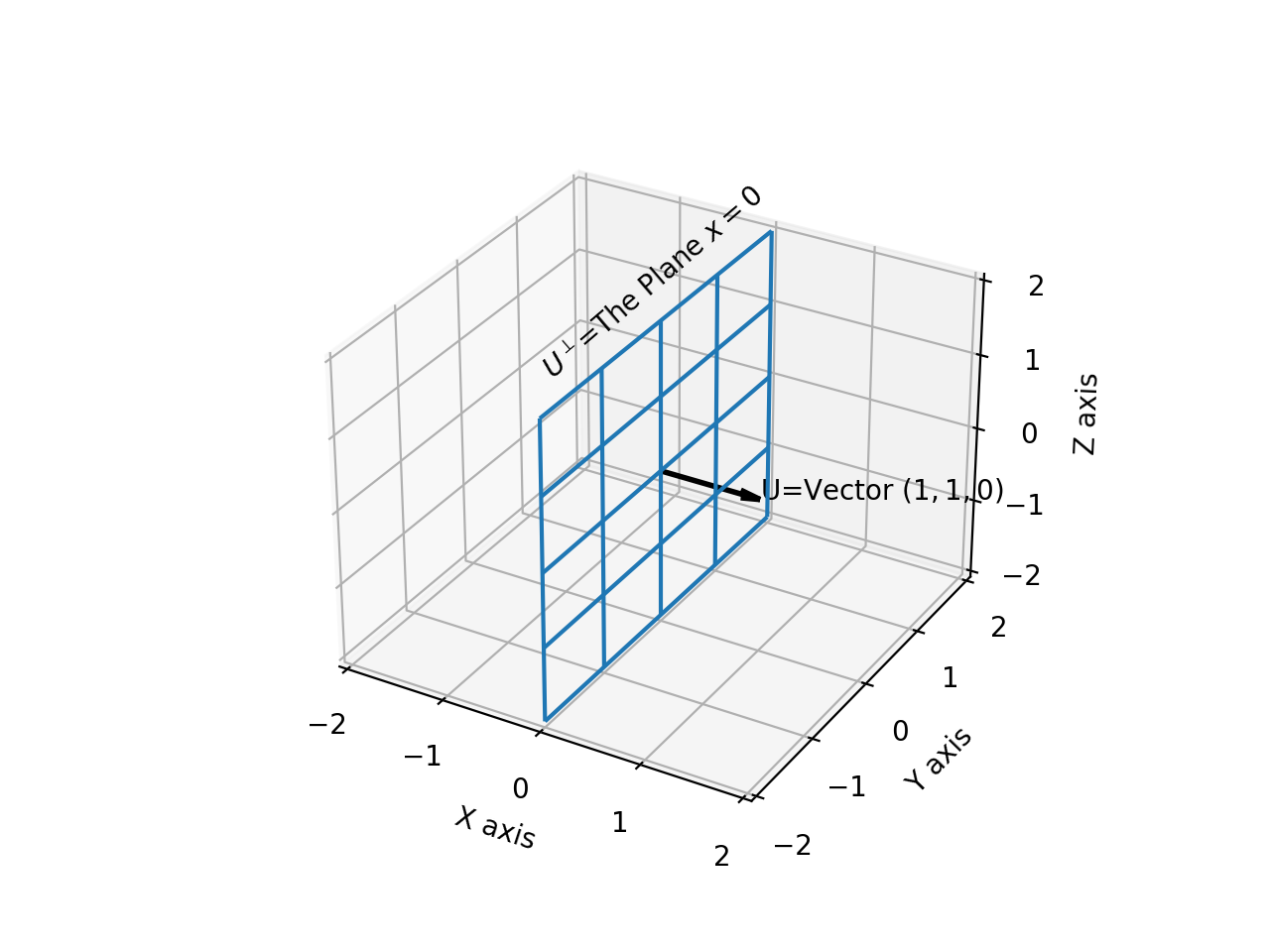
We illustrate this with a simple motivating example, but without proof. If \(\vec{U}=(1,0,0)\), then its orthogonal complement \(U^{\perp}\) is the plane \(x=0\), as shown below:

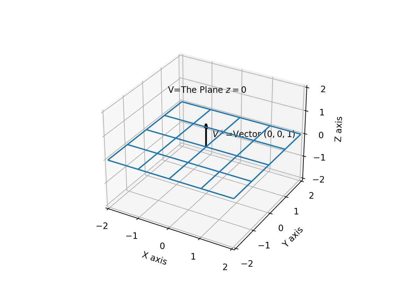
If \(V\) is the plane \(z=0\), then its orthogonal complement is \(\vec{V^{\perp}}=(0,0,1)\), as shown below:

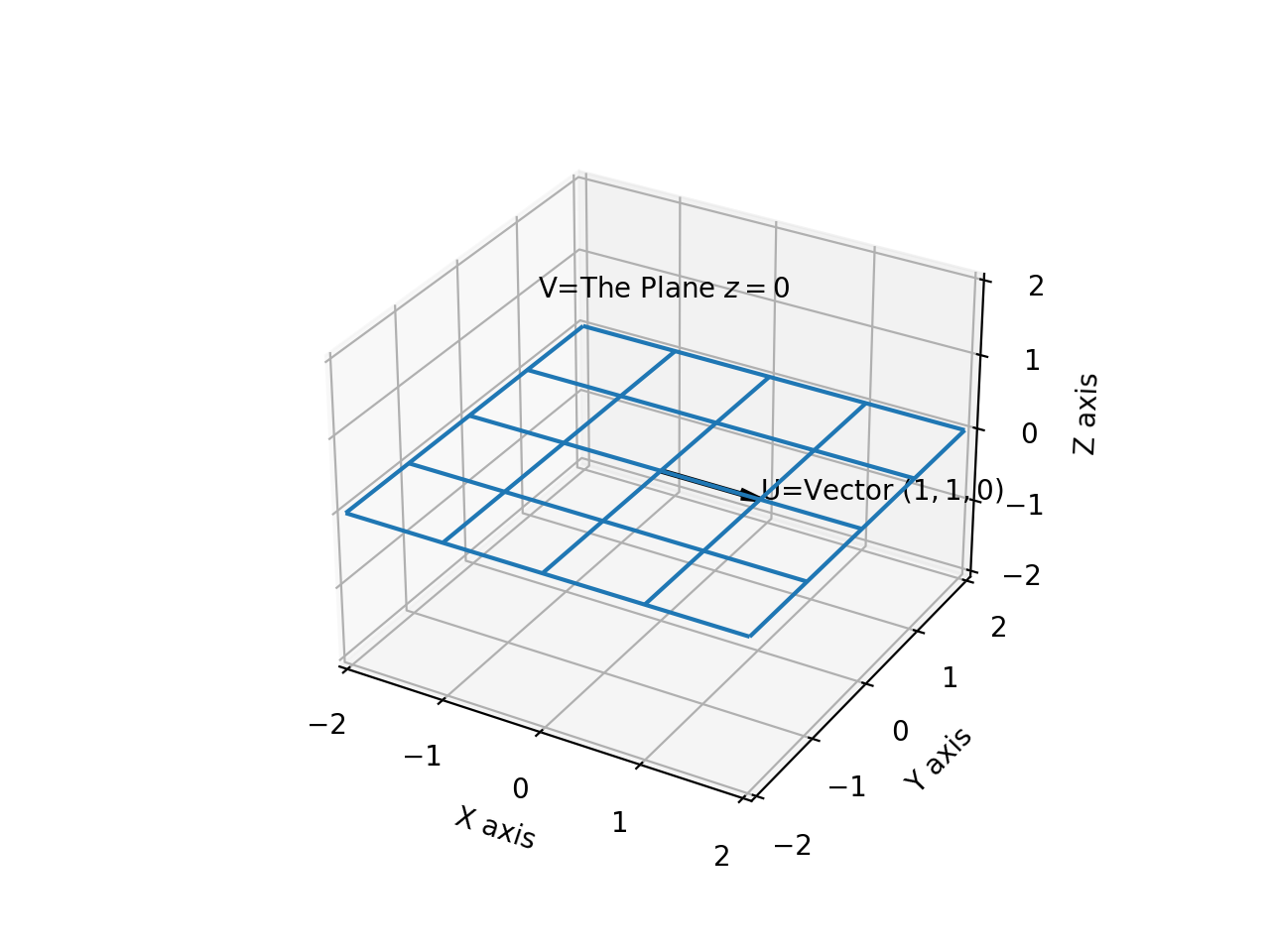
Now, the relation \(\mathbf{U\subset V}\) clearly holds, since the vector \(\vec{U}=(1,0,0)\) exists in the plane \(V=z=0\), as shown below:

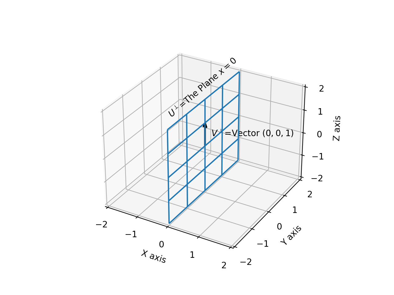
Similarly, the relation \(\mathbf{U^{\perp}\supset V^{\perp}}\) clearly holds, since \(U^{\perp}=x=0\) contains the vector \(\vec{V^{\perp}}=(0,0,1)\), as shown below:

This validates the Subset Rule.

Graphs and Level Sets

Optimisation problems boil down to maximising (or minimising) a function of (usually) multiple variables. The form of the function has a bearing on how easy or hard the solution might be. This section introduces some terminology that further discussion will refer to, and it is best to not admit any ambiguity in some of these terms.

Graph of a Function

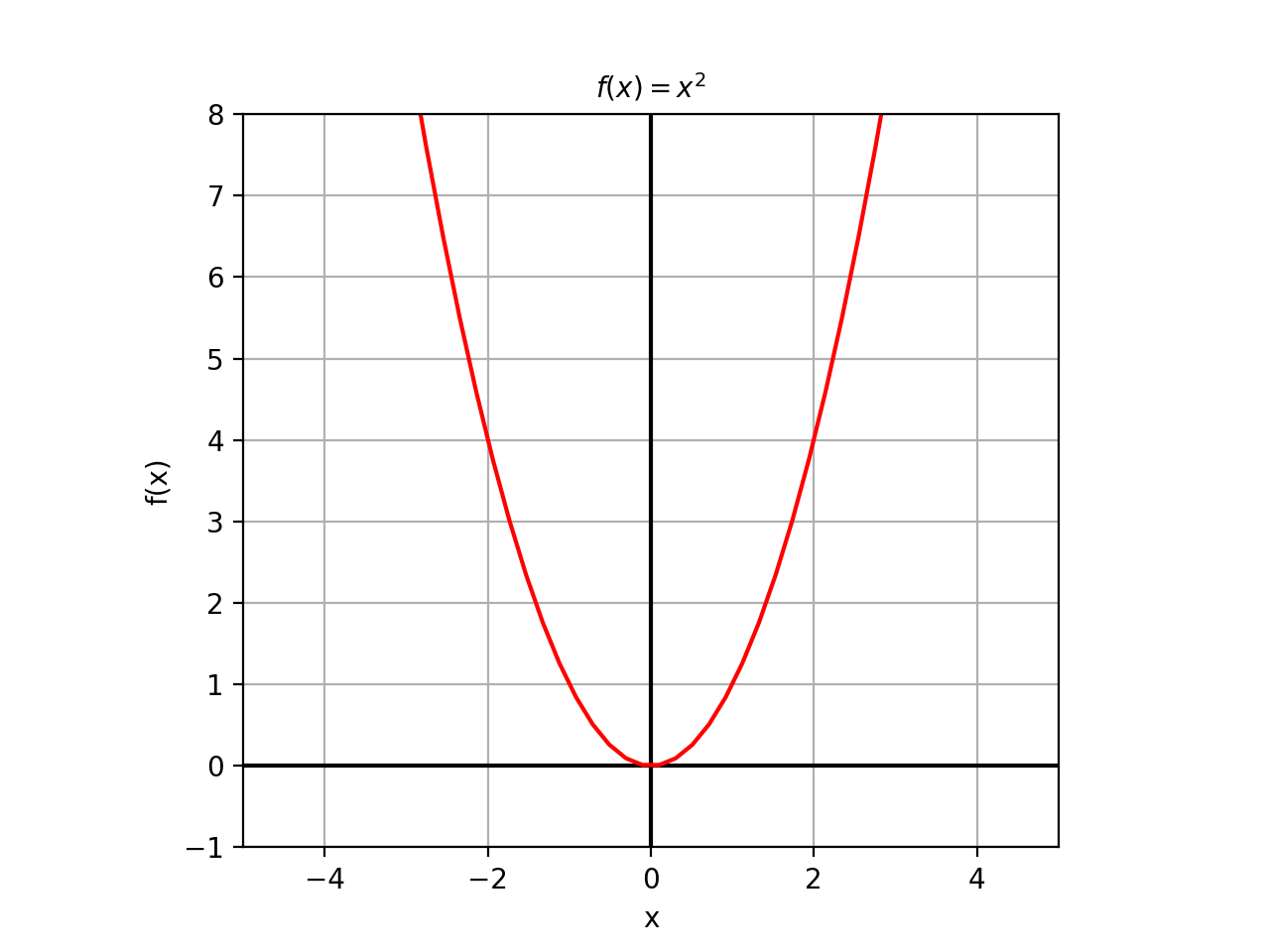
Consider the function \(f(x)=x^2\). By itself, it represents a single curve. This is a function of variable. This is the picture of what it looks like:

However, consider what the function \(g(x)=(x,f(x))\) looks like. This notation might seem unfamiliar – after all, isn’t a function supposed to output a single value? – but we have already dealt with functions that return multiple values; we just bundled them up in matrices. So it is the case in this scenario: \(g(x)\) takes in a value in \(\mathbb{R}\) and returns a matrix (usually a column vector, for the sake of consistency) of the form:

\(\begin{bmatrix} x \\ f(x) \end{bmatrix}\). This function \(g(x)=(x,f(x))\) is called the graph of the function \(f(x).\)Later on, when we introduce vector-valued functions, \(x\) and \(f(x)\) will themselves be column vectors in their own right.

Level Set of a Function

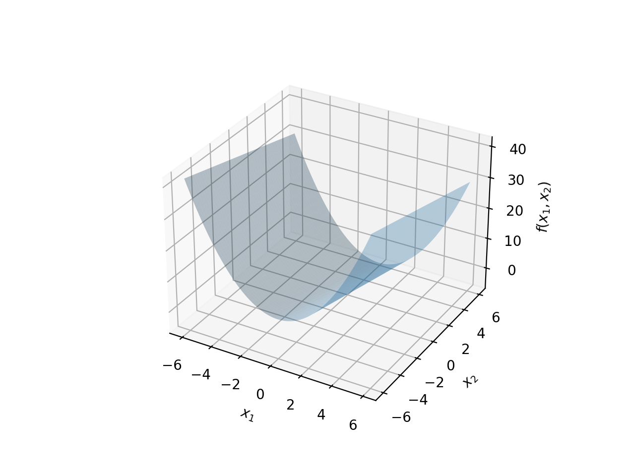
Consider the function \(f(x_1,x_2)=x_1^2-x_2\). This is a function of two independent variables \(x_1\) and \(x_2\). Note that this function is very similar to \(y=x^2\) (which can be rewritten as \(x^2-y=0\)), except there is no constraint on the output value. If we wish to observe the shape of this function, we will need to look at it in 3D: two dimensions for the independent variables, and the third for the output of the function \(f(x_1,x_2)\).

Together, this will form a two dimensional surface in 3D space; the picture below shows what this surface would look like.

The surface above is a surface because there is no constraint. However, you can think of this surface as the family of all possible parabolas of the form \(x^2-y=C\), where we have let \(C\) unspecified. Each value of \(C\) gives us one parabola in this family. Let’s look at this in 2D first in the image below.

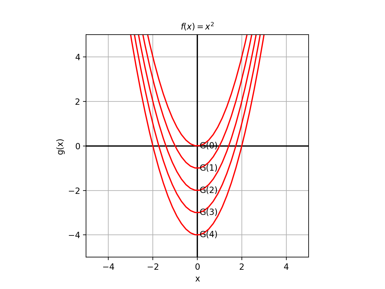
Each member of this family of parabolas is obtained by fixing \(C\) to a specific value. This fixing function is called the Level Set of the function \(f(x)\). We denote it here by \(G(C)\), where \(C\) is the constant which selects a particular parabola from this family. Thus, \(G(2)\) results in the equation \(x_1^2-x_2=4\).

The above diagram does not give us the full picture. Remember, the actual value of \(C\) is not pictured here, because it exists in the third dimension. We need to go back to our parabola surface we pictured earlier. We will do the same thing, plot some sample members of this family, but this time we will also position them along the Z-axis based on what value \(f(x)\) assumes (which is of course \(C\), since we are explicitly fixing for each level set/parabola).

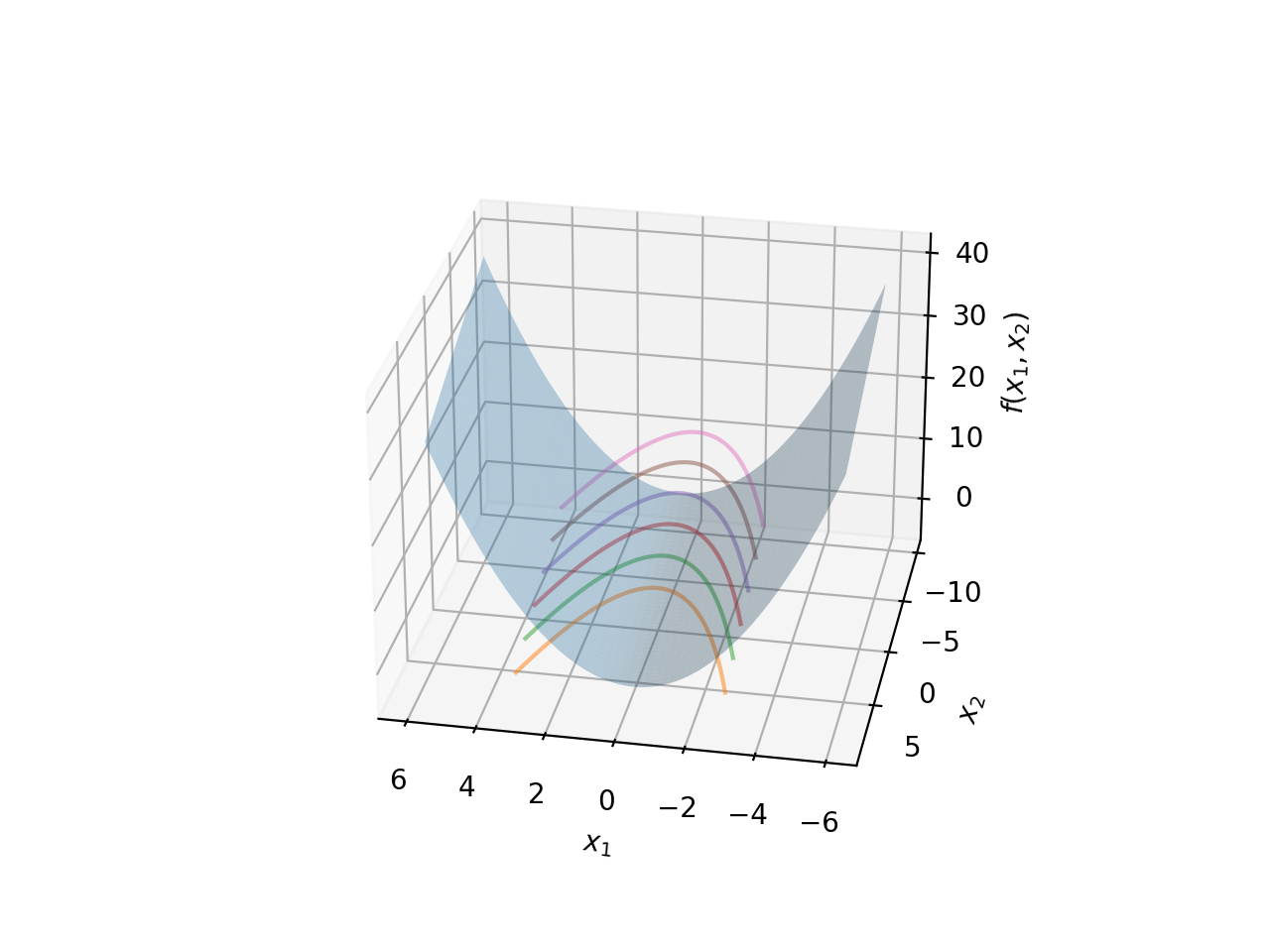
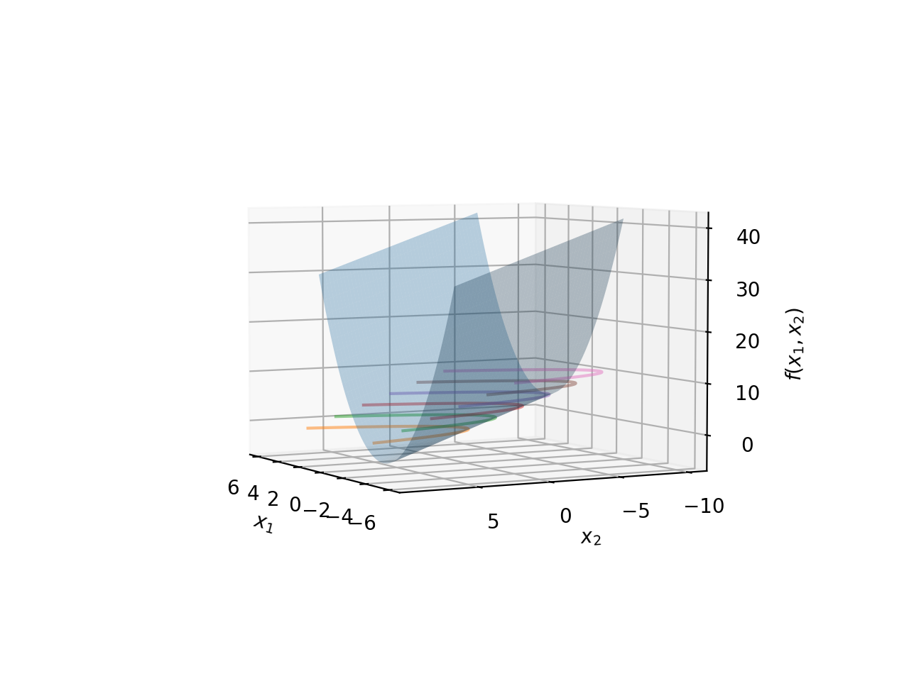
Both are the same graph, just rotated a bit to give you a better idea of where these level sets lie in space in relation to the surface of the family of parabolas. As you can see, each level set is fixed at a particular \(z\) value because we are fixing \(C\). Each level set always lies on this surface. In essence, each level set is a horizontal cross-section of the full surface, with the position of the cut specified by fixing \(C\).

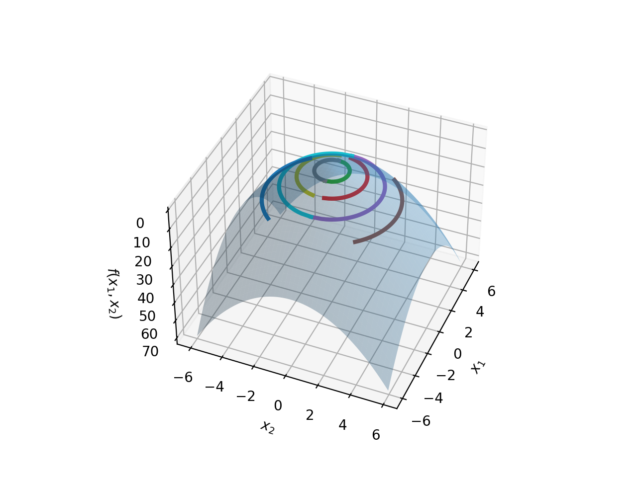
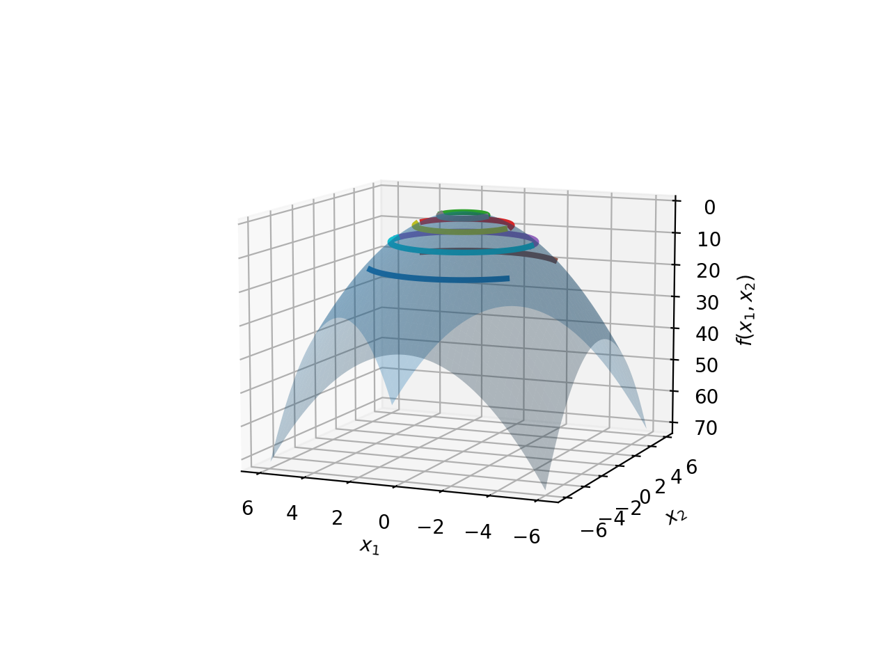
A circle is usually a better candidate for demonstrating this visually, thus we will repeat the same illustration with the function \(f(x)=x^2+y^2\). This defines the family of circles centered at \((0,0)\) with all possible radii \(C\in\mathbb{R}\).

As usual, picking a particular radius fixes a level set on the surface of this family of circles. The image below shows the situation:

Let’s put Level Sets into action. Let’s take a familiar exercise, and apply our understanding of level sets to it, that will allow us to interpret the solution with our new-found knowledge.

Exercise: Find the tangent line to the curve \(y=x^2+4\), and \(x=3\).

This is the level set of a function \(g(x,y)=y-x^2\), with \(G(4)\), if we assume \(G\) to be the level set function.

Let’s work with just \(g(x,y)\). Differentiating partially:

\[Dg(x,y) = \left[ \frac{\partial g(x,y)}{\partial x} \frac{\partial g(x,y)}{\partial y} \right] = [-2x \hspace{1cm} 1]\]

This immediately gives us the vector normal to the curve at a given \((x,y)\). Remember, \(g(x,y)\) is a surface, so the differentiation gives us a tangent plane. The tangent plane is represented by its normal vector, hence the vector is normal to the curve. The normal vector at \(x=3\) is \(\begin{bmatrix} -6 \\ 1 \end{bmatrix}\)

However this is not the tangent line. If you consider the actual line that this normal vector represents (actually, one of the lines, you can get infinitely many lines by translation, we discuss this below), that is: \(\mathbf{y-6x=0}\), we see that it passes through the origin, and is definitely not tangent to the curve, as shown in the picture below. It has the correct slope, but it is displaced.

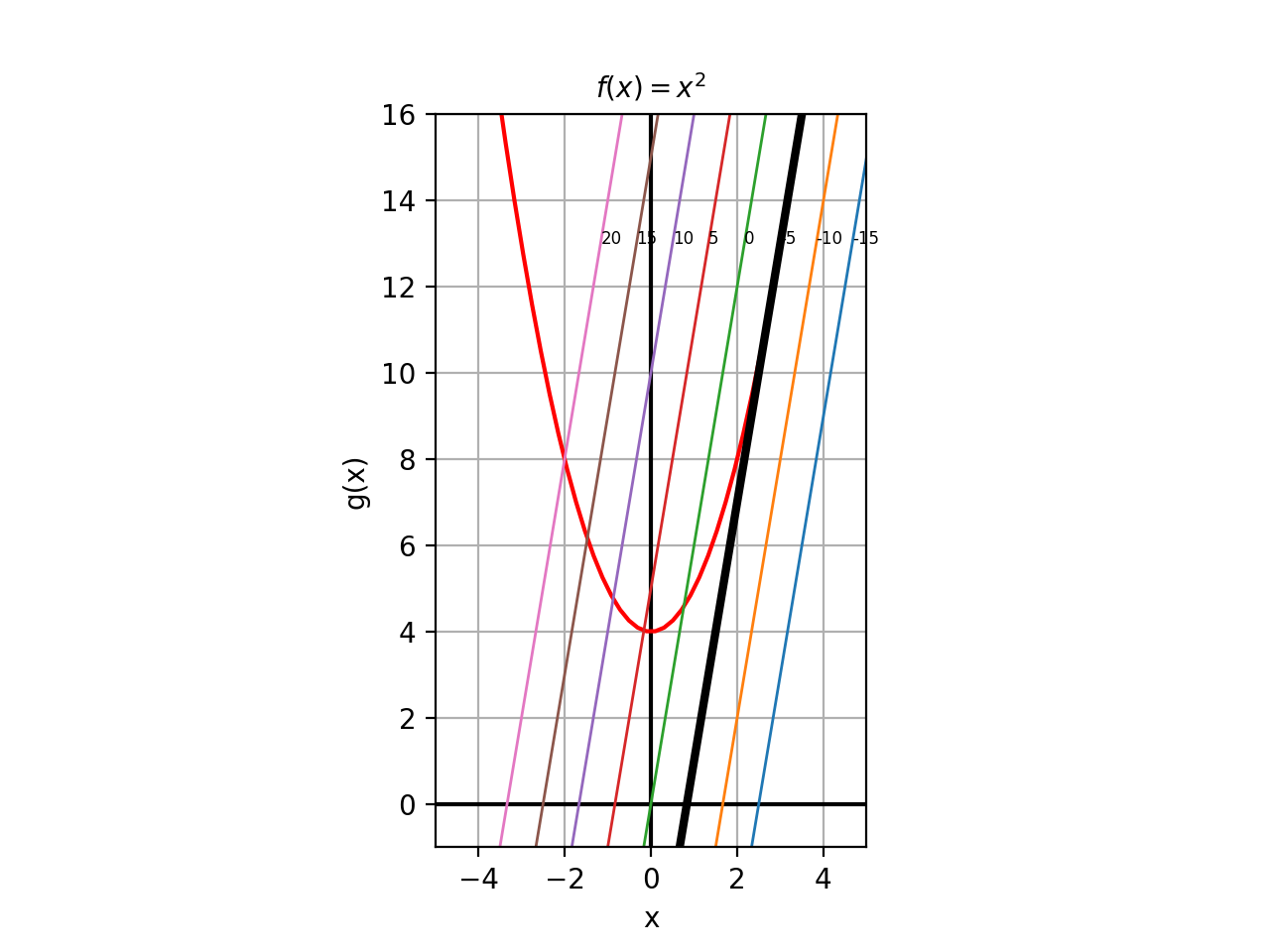
The reason is that \(\mathbf{t(x,y)=y-6x}\) represents a family of tangent lines; each level set, fixed by a value of \(c\) represents a particular member of that family. For our curve \(y-x^2=4\), the tangent line and this curve is the same graph only at \((3,13)\), which is the point where the tangent line should touch. This means that we can find the level set parameter we are seeking, by substituting \((3,13)\) into \(t(x,y)=y-6x\). This gives us:

\[t(3,13)=13-18=-5\]

Plugging in -5 as the level set value for the function gives us \(\mathbf{y-6x=-5}\), which is the correct tangent line. This line is shown in bold in the plot above.

We could have solved it taking a slightly different, possibly more general, approach. We know that the tangent exists at \((3,13)\). We know that \(y\) can be expressed in terms of \(x\) as \(y=x^2+4\). Thus, any point in the neighbourhood of \((3,13)\) will still lie on the tangent line, and must satisfy the following:

\[\frac{y-13}{x-3}=\frac{\partial y}{\partial x} \\ \Rightarrow y-13=\frac{\partial y}{\partial x}(x-3)\]

Well, \(y\) does not depend upon anything other than \(x\), so taking the partial is the same as your normal derivative, which is \(\frac{dy}{dx}=6\). Substituting this back into the above identity, we get:

\[y-13=6(x-3) \\ \Rightarrow y-13=6x-18 \\ \Rightarrow y-6x-=-5 \\ \Rightarrow \mathbf{y-6x-=-5}\]

This confirms the previous calculation.

This second line of finding out a tangent line will prove more useful, when we extend the discussion to tangent spaces in higher dimensions. Keep this at the back of your mind.

There is one more point that I want to make which will be important as it will be restated in the proof for points constrained to a manifold. The function \(g(x)=y=x^2\) represents \(y\) in terms of \(x\). The differential of this function is obviously \(Dg(x)\).

\(Dg(x)\) thus is the mapping which relates the \(y\) coordinate to the \(x\) coordinate for all points on the tangent line. Thus, the graph of \(Dg(x)\) is the tangent line (more generally the tangent space) for this particular curve.

Gradients and Jacobians

I will touch on Jacobians lightly because a significant part of what is to come in this article, will differentiate functions with respect to vectors, very often. Jacobians are the application of partial derivatives on multiple vector-valued functions, i.e., they accept vectors as inputs. To make this more concrete, and show the most general case for matrices, we take \(m\) functions, each taking as input an n-dimensional vector. Thus, our initial matrix will be an \(m \times n\) matrix, like so:

Taking the Jacobian of \(F\) is partial differentiation of \(f_i\)with respect to each \(x_i\), and repeating this for all functions in the matrix.

\[J_XF=\begin{bmatrix} \frac{\partial f_1}{\partial x_1} && \frac{\partial f_1}{\partial x_2} && \cdots && \frac{\partial f_1}{\partial x_n} \\ \frac{\partial f_2}{\partial x_1} && \frac{\partial f_2}{\partial x_2} && \cdots && \frac{\partial f_2}{\partial x_n} \\ \frac{\partial f_3}{\partial x_1} && \frac{\partial f_3}{\partial x_2} && \cdots && \frac{\partial f_3}{\partial x_n} \\ \vdots \\ \frac{\partial f_m}{\partial x_1} && \frac{\partial f_m}{\partial x_2} && \cdots && \frac{\partial f_m}{\partial x_n} \\ \end{bmatrix}\]

where the subscript \(X\) indicates we are differentiating with respect to the vector \(X=(x_1,x_2,...,x_n)\).

Tangent Spaces

The exercise in the section on Level Sets leads directly from the one-dimensional case to a discussion on Tangent Spaces in higher dimensions. Remember the equation to find the tangent space in one dimension, where we represented one variable in terms of the other? I reproduce it below for reference:

\[y-y_0=\frac{dy}{dx}(x-x_0)\]

Here, we have simply replaced the concrete values with \((x_0,y_0)\). This is usually referred to as the parametric form of a linear function. It tells you how much \(y\) when you change \(x\) by a certain value. Specifically, it also tells you how much \(y\) changes by, when you change \(x\) by 1.This value is also, unsurprisingly, the slope of the linear function, represented here as \(\frac{\partial y}{\partial x}\). Any vector on this linear function can be represented as \(\begin{bmatrix}1 \\ \frac{dy}{dx}\end{bmatrix}.t\)

Now, consider any equation of three variables. As an example:

\[x+2y+3z=0\]

Here, we can represent \(z\) as a function of \((x,y)\), like so:

\[z=-\frac{x+2y}{3}\]

We have essentially moved up one dimension from the previous example, where one variable is now expressed in terms of two variables, instead of one. If we wish to find the tangent space for this, we can use the same concept, except that this time partial differentiation will make sense, since you have two dependent variables, so you take the partial derivative for each of them separately. So, we can write:

\[z-z_0=\begin{bmatrix} \frac{\partial z}{\partial x} && \frac{\partial z}{\partial y} \end{bmatrix} \begin{bmatrix} x-x_0 \\ y-y_0 \end{bmatrix}\]

Thus, similar to the previous case, if we denote \(g(x,y)=\begin{bmatrix} \frac{\partial z}{\partial x} && \frac{\partial z}{\partial y} \end{bmatrix}\), \(g(x,y)\) denotes a mapping from the independent variables \(x\) and \(y\) to \(z\). Stated more generally, \(g(x,y)\) is a mapping from \(\mathbb{R}^2\) to \(\mathbb{R}\). As before, the graph of \(g(x,y)\) is the tangent space. Remember, a graph is simply the set of all inputs (in this case, \(x\) and \(y\)) and their corresponding outputs (in this case \(z\)); thus the graph of \(g(x,y)\) is simply all the \((x,y,z)\) tuples which lie on the tangent space.

We can extend this easily enough to n-dimensional space, where one variable can be expressed in terms of \(n-1\) independent variables. That is, if \(x_n=g([x_1, x_2,..., x_{n-1}])\)

\[x_n=\begin{bmatrix} \frac{\partial g}{\partial x_1} && \frac{\partial g}{\partial x_2} && ... && \frac{\partial g}{\partial x_{n-1}} \end{bmatrix} \begin{bmatrix} x_1 \\ x_2 \\ x_3 \\ \vdots \\ x_{n-1} \end{bmatrix}\]

This is a single linear equation. We will have more to say about linearity in nonlinear curves in another article. Now we extend this to multiple equations. Before we do that though, let’s consider a simple motivating example to make the intuition about independent and dependent variables in a linear system of equations, more solid.

Consider two equations:

\[x+y+z=0 \\ x+2y+3z=0\]

What is the solution to this set of equations? Let’s use the row reduction technique to find the pivots. We first write out the system of linear equations as a matrix.

\[\begin{bmatrix} 1 && 1 && 1 \\ 1 && 2 && 3 \end{bmatrix}\]

Let’s now convert to reduced row echelon form, first subtracting \(R_1\) from \(R_2\)

\[\begin{bmatrix} 1 && 1 && 1 \\ 0 && 1 && 2 \end{bmatrix}\]

Now, we subtract \(R_2\) from \(R_1\) to get:

\[\begin{bmatrix} 1 && 0 && -1 \\ 0 && 1 && 2 \end{bmatrix}\]

We have arrived at the row reduced echelon form. We see that we have two pivots, \(x\) and \(y\); rank of the matrix is 2.

\[x-z=0 \\ \Rightarrow x=z \\ y+2z=0 \\ \Rightarrow y=-2z\]

Thus, we have one free variable (\(z\)), which can be used to express \(x\) and \(y\). Note that the rank of the matrix, which is 2, and the number of variables, which is 3. As a general rules, if we have a system of \(n-k\) equations for \(n\) variables, there are \(k\) free variables (parameters), and the remaining \(n-k\) variables can be expressed in terms of the \(k\) parameters.

You will have also noticed that the final result is the parametric form of a line in 3D space. This is not surprising, because the solution represents the intersection of two planes.

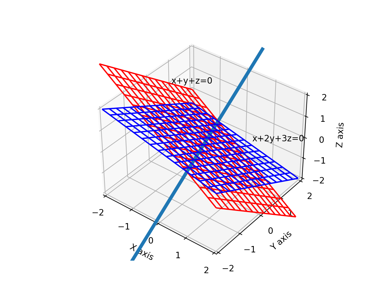
We can say that this line (\(x=z,y=-2z\)) is a manifold. The definition of a manifold involves several conditions that need to be satisfied, and they are related to ideas about differentiability and local linearity. We will visualise some of those ideas in the next article. The important thing to connect this material with Machine Learning is that an optimisation problem defines a set of constraints. These constraints limit the area where an optimal solution can exist. These constraints are what we represent by \(n-k\) equations. Note that, in the usual case of optimisation, we will have more variables than equations, i.e., \(n>k\). In this context, we may call the manifold, a constraint manifold.

Thus, if we have a system of \(\mathbf{n-k}\) equations, assuming this linear system has maximum possible rank, i.e., all the column vectors are linearly independent, we will have \(n-k\) pivots. This implies that there exist \(\mathbf{k}\) free variables (parameters) which can be used to express the remaining \(n-k\) dependent variables.

The matrix of these functions can be represented as:

\[F(X)=\begin{bmatrix} f_1(x_1,x_2,...,x_n) \\ f_2(x_1,x_2,...,x_n) \\ f_3(x_1,x_2,...,x_n) \\ \vdots \\ f_{n-k}(x_1,x_2,...,x_n) \\ \end{bmatrix}\]

Then, we may extend our single-function expression of the slope, and write as below:

\[\begin{bmatrix} x_{k+1} \\ x_{k+2} \\ x_{k+3} \\ \vdots \\ x_{n-k} \end{bmatrix} =\begin{bmatrix} \frac{\partial g_1}{\partial x_1} && \frac{\partial g_1}{\partial x_2} && ... && \frac{\partial g_1}{\partial x_k} \\ \frac{\partial g_2}{\partial x_1} && \frac{\partial g_2}{\partial x_2} && ... && \frac{\partial g_2}{\partial x_k} \\ \vdots \\ \frac{\partial g_{n-k}}{\partial x_1} && \frac{\partial g_{n-k}}{\partial x_2} && ... && \frac{\partial g_{n-k}}{\partial x_k} \\ \end{bmatrix} \begin{bmatrix} x_1 \\ x_2 \\ x_3 \\ \vdots \\ x_k \end{bmatrix}\]

The above says that \(n-k\) variables can be expressed as a linear transformation of \(k\) variables. Each entry in the output vector is expressed as a combination of multiple input variables, and are related to each input variable by the “slope” obtained through the partial derivative.

This is a generalisation we say earlier, of a single output variable expressed through a single input variable, related to it through a single function. In that example, that function was the slope of the graph, obtained by differentiating the equation of the curve; thus the graph of that function was the tangent space.

So it is with this complicated-looking expression: it represents the tangent space of a manifold which is defined by \(n-k\) equations.

One question that will inevitably arise is: how does this set of linear equations ultimately motivate optimisation on complex manifolds? The Implicit Function Theorem answers this question, and is the jumping-off point for the next post on Vector Calculus.

---