Vector Calculus: Lagrange Multipliers, Manifolds, and the Implicit Function Theorem

Avishek Sen Gupta on 24 April 2021

---

In this article, we finally put all our understanding of Vector Calculus to use by showing why and how Lagrange Multipliers work. We will be focusing on several important ideas, but the most important one is around the linearisation of spaces at a local level, which might not be smooth globally. The Implicit Function Theorem will provide a strong statement around the conditions necessary to satisfy this.

We will then look at critical points, and how constraining them to a manifold naturally leads to the condition that the normal vector of the curve to be optimised, must also be normal to the tangent space of the manifold.

We will then restate this in terms of Lagrange multipliers.

Note: This article pulls a lot of understanding together, so be sure to have understood the material in Vector Calculus: Graphs, Level Sets, and Linear Manifolds, before delving into this article, or you might get thoroughly confused.

Definition of a Manifold

Let us make precise the definition of a manifold now.

We’ve looked at a system of \(k\) linear equations of \(n\) variables, where \(n-k\) variables were expressed in terms of \(k\) independent variables. If we remove the requirement of these equations being linear, then the solution space, i.e., the set of points \((x_1, x_2,..., x_n)\) which satisfy this system, constitutes a k-manifold in \(\mathbb{R}^n\).

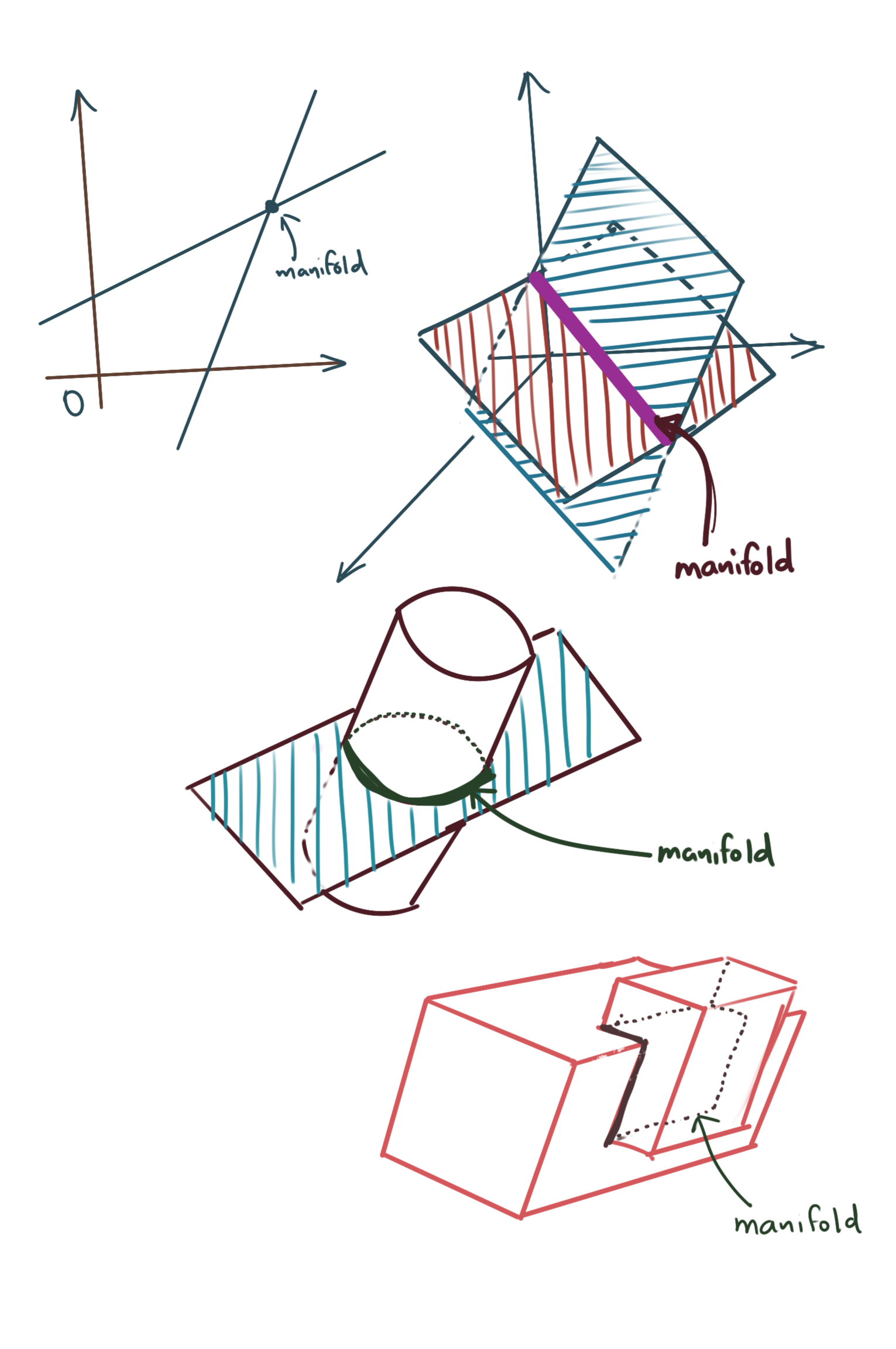
• For a single equation, a manifold is simply the graph of that function.
• For multiple equations, a manifold is essentially the set of points which satisfy all of those equations. For example:
  • If we had two equations of intersecting lines in \(\mathbb{R}^2\), then the manifold would simply be the point of intersection.
  • If we had two equations of intersecting planes in \(\mathbb{R}^3\), the manifold would be the line of intersection of those two planes.
  • All vector subspaces are manifolds.

The structure of this article follows this sequence.

• Constrained Critical Points in Two Dimensions
• Constrained Critical Points in the General Case
• Lagrangian Formulation and Proof
• Extension to Nonlinear Constraints: Implicit Function Theorem

We start with two important preliminaries.

• Function Composition
• Chain Rule and Functions as Objects

Preliminary: Function Composition and Functions as Objects

Let us assume that:

\[f(x,y)=xy \\ y=g(x)=x^2\]

Then the notation \(\mathbf{F=f\circ g}\) represents function composition, where represents a function \(F\) which has the same output as \(f(x,g(x))\) (in this example). Also note that \(F\) is a function of only \(x\). In texts, \(f(x,y)\) is written as \(f(x,g(x))\) and is equivalent to the above form.

Do not let the fact that there is a function in the parameter of \(f\) confuse you; treat it as you would any other variable. If you know the actual expression \(f(x,g)\), you can differentiate with respect to \(g\) if needed. After all, \(g(x)\) is essentially \(y\).

Writing it as \(f(x,g(x))\) is notational shorthand for expressing that \(y\) is not really a free variable, it is expressed in terms of \(x\). Moreover \(D_xF(x)\) is the same thing as writing \(Df(x,g(x))\).

We can borrow our intuition of function pipelines in programming to make sense of this: an input \(x\) enters \(g(x)\), comes out as some output, which is then fed to the \(y\) parameter of \(f(x,y)\). The \(x\) parameter is already available, so it gets applied for free (actually, while programming, you can’t say things like “gets applied for free”, you actually have to do the necessary plumbing to allow \(x\) to reach \(f(x,y)\)).

Note that the composite function \(F(x)\) takes in only one input, \(x\). This is because the first function that is applied is \(g(x)\). You do not need to specify a \(y\) – in fact, you should not – because the value of \(y\) is constrained to be (in this instance) \(x^2\).

You can do symbolic manipulation to directly substitute \(g(x)\) into \(F(x)\) to get \(F(x)=x.x^2=x^3\). Either way, that’s how function composition works. We introduce this because it will be used to build in the constraints for our optimisation problem, and we will see how taking derivatives of composed functions translates to the dot product of linear transformations.

Preliminary: Chain Rule

Let us continue with the above example. Assume that:

\[f(x,y)=xy \\ y=g(x)=x^2\]

Then the notation \(F=f\circ g\) represents function composition, where \(F(x)=f(x,g(x))\), as we have already stated.

Now, if we wanted to find \(D_xf(x,g(x))\), it is trivial to see that substituting \(x^2\) for \(y\) in \(f(x,y)\) gives us \(f(x)=x^3\), therefore:

\[D_xf(x,g(x))=3x^2\]

However, let’s look at the Chain Rule of differentiation for the above \(f(x,y)\), because in our proofs, the actual form of \(f(x,y)\) and \(g(x)\) will not be available, and thus we will have to use the Chain Rule to express any results. We have only one free variable for this composite function, i.e., \(x\), so we may write:

\[D_xf(x,g)=\frac{\partial f(x,g)}{\partial x} \\ =\frac{df(x, g)}{d{[x\hspace{3mm} g]}^T}.\frac{d{[x\hspace{3mm} g]}^T}{dx} \\\]

Let’s denote \(\Phi (x)=\begin {bmatrix}x \\ g\end{bmatrix}\). \({[x \hspace{3mm} g]}^T\) is a vector so we are partially differentiating \(f(x,y)\). In our example above, we can write for the first term, and substitute:

\[\frac{df(x,g)}{d[x \hspace{3mm} g]}=\left[\frac{\partial f(x,g)}{\partial x} \hspace{3mm} \frac{\partial f(x,g)}{\partial g} \right] \\ \Rightarrow D_xf(x,y)=\left[\frac{\partial f(x,g)}{\partial x} \hspace{3mm} \frac{\partial f(x,g)}{\partial g} \right].\frac{d\Phi (x)}{dx}\]

For the second term, we may write:

\[\frac{d{[x \hspace{3mm} g]}^T}{dx}=\begin{bmatrix} 1 \\ \frac{dg}{dx} \end{bmatrix} \\ \Rightarrow D_xf(x,g)=\left[\frac{\partial f(x,g)}{\partial x} \hspace{3mm} \frac{\partial f(x,g)}{\partial g} \right].\begin{bmatrix} 1 \\ \frac{dg}{dx} \end{bmatrix} \\ = \frac{\partial f(x,g)}{\partial x} + \frac{\partial f(x,g)}{\partial g}\frac{dg}{dx}\]

Only now do we need to unroll \(g(x)\) to look at the specific form this derivative takes. We can write the following:

\[\frac{dg}{dx}=2x \\ \frac{\partial f(x,g)}{\partial x}=g \\ \frac{\partial f(x,g)}{\partial g}=x\]

Substituting these values back into the expression for \(D_xF(x)\), we get:

\[D_xf(x,g)=g+x.2x=g(x)+2x^2 \\ = x^2+2x^2 \\ = 3x^2\]

Yes, that was a complicated way of computing the same result we got earlier, but I want you to see the mechanics involved in applying the Chain Rule in the case of partial derivatives.

Constrained Critical Points in Two Dimensions

The previous example can be reused to illustrate the concept of constrained critical points in two dimensions. Let us revisit the intermediate expression we used, namely:

\[D_xf(x,g)=\left[\frac{\partial f(x,g)}{\partial x} \hspace{3mm} \frac{\partial f(x,g)}{\partial g} \right].\frac{d\Phi (x)}{dx}\]

If you notice carefully, the expression \(\left[\frac{\partial f(x,g)}{\partial x} \hspace{3mm} \frac{\partial f(x,g)}{\partial g} \right]\) exactly represents the gradient operator \(\nabla f(x,g(x))\).

Furthermore, look at \(\frac {d\Phi (x)}{dx}=\begin{bmatrix}1 \\ \frac{dg}{dx}\end{bmatrix}\). We can recognise this as the parametric form of the line \(\mathbf{y=g'(x).x}\). This is because any vector on the tangent can be represented as \(\begin{bmatrix}1 \\ \frac{dg}{dx}\end{bmatrix}.t\).

As a consequence, this is the tangent space of \(g(x)\). If we represent \(\frac {d\Phi (x)}{dx}\) as \(T_x\) (the tangent space), we can rewrite the identity as:

\(D_xf(x,g)=\nabla f(x,g(x)).T_x\)

Important Note: Note that \(T_x\) is not the normal vector to the tangent, but the actual vector along the tangent.

The picture below shows the situation. The function \(f(x,y)=xy\) is the function to be optimised. However, setting \(y=x^2\), and substituting it into \(f(x,y)\) so that it becomes \(f(x,g(x))\) immediately constrains the y-coordinate to always be such that for any \(x\), the point is always forced to move along the curve \(y=x^2\), regardless of which level set of \(f(x,g(x))\) is chosen.

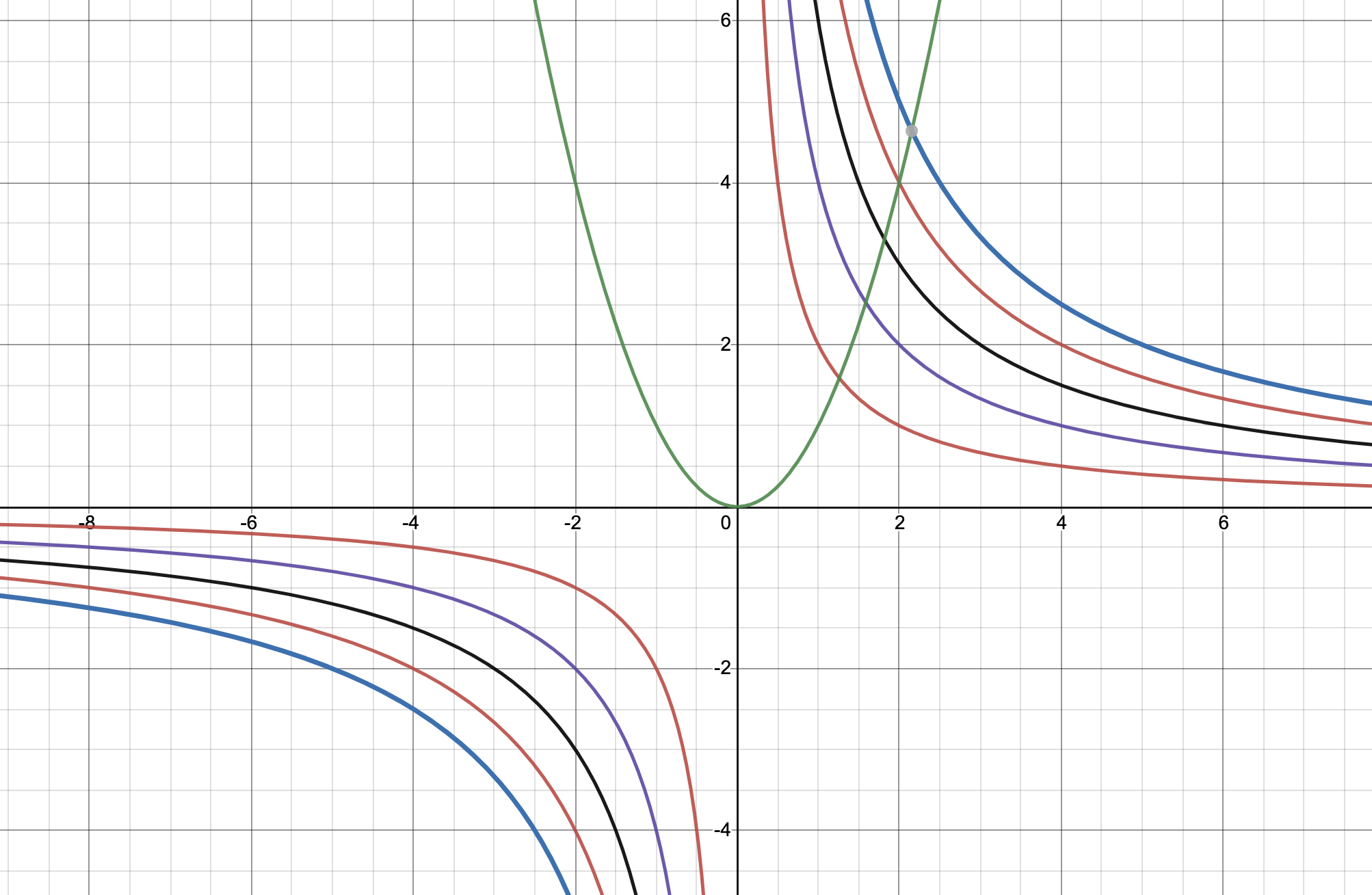
Note: The above example isn’t the best example because attempting to find a constrained critical point in this situation will result in \((0,undefined)\) on the curve, but the identities we derive here, still hold. We solve a more feasible problem next.

If we have a point \(P\) which satisfies \(g(x)\), i.e., has the coordinates \((x_0, g(x_0))\), then the following holds:

\(D_xf(P)=\nabla f(P).T_x\)

The above expression represents the dot product of the gradient vector and the tangent vector at a point P which exists on the curve of the function defined by \(f(x,y)=xy\) and satisfies the constraint \(g(x)=x^2\).

Let us look at a problem with a proper solution.

\[f(x)=xy \\ y=g(x)=y=4-x\]

Let’s use the result we derived above. We have:

\[\nabla f=\begin{bmatrix}y && x\end{bmatrix} \\ \frac{d\Phi}{dx}=\begin{bmatrix}1 \\ -1\end{bmatrix}\]

Multiplying the two, we get:

\[D_xf=\nabla f.T_x=\begin{bmatrix}y && x\end{bmatrix}.\begin{bmatrix}1 \\ -1\end{bmatrix}=y-x=(4-x)-x=4-2x\]

Setting the above to zero, we get:

\[4-2x=0 \Rightarrow x=2 \Rightarrow y=2\]

which is the solution we seek. Substituting \(x=2\) back into \(f(x,y)=xy\) gives us the correct level set, i.e., \(xy=4\). The solution is shown below.

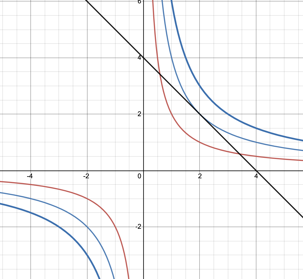
The constrained critical point is \((2,2)\). Note that this is different from finding an intersection between two curves. There are an infinite number of \(xy=C\) equations which can intersect with \(y=x^2\). For example, \(xy=2\) intersects with the constraint line in two places, But that does not maximise the value of \(xy\).

You will have also noticed that the curve containing the constrained critical point is tangent to the constraint curve (straight line, in this case). This is not a coincidence, as we will see when we get to the generalised, higher-dimensional case.

The above simple two-dimensional case will serve as our starting point. We now generalise in two conceptual directions.

Generalisation to Multiple Constraints

Recall what we spoke about systems of linear equations in Vector Calculus: Graphs, Level Sets, and Linear Manifolds. Specifically, if there are \(n\) variables, and \(n-k\) equations, we can parametrically specify \(n-k\) variables in terms of the other \(k\) free variables.

We can generalise the above dot product derivation for this general case. Before we do this, in order to avoid the ugly-looking \(n-k\) expression, we restate the above as:

If there are \(N\) variables, and \(n\) equations, we can parametrically specify \(n\) variables in terms of the other \(m\) free variables. Also, obviously, \(m+n=N\). Let the independent variables be \(U=(u_1, u_2, u_3,...,u_m)\), and the dependent variables be \(V=(v_1, v_2, v_3,...,v_m)\)

Now we write:

\[G(U)=\begin{bmatrix} u_1 \\ u_2 \\ u_3 \\ \vdots \\ u_m \\ \phi_1(u_1, u_2, u_3, ..., u_m) \\ \phi_2(u_1, u_2, u_3, ..., u_m) \\ \phi_3(u_1, u_2, u_3, ..., u_m) \\ \vdots \\ \phi_n(u_1, u_2, u_3, ..., u_m) \end{bmatrix} =\begin{bmatrix} u_1 \\ u_2 \\ u_3 \\ \vdots \\ u_m \\ \phi_1 \\ \phi_2 \\ \phi_3 \\ \vdots \\ \phi_n \end{bmatrix} \\ \\ \Rightarrow G(U)=(U,V) \\ f(u_1, u_2, u_3, ..., u_m, v_1, v_2, v_3, ..., v_n)\]

You should be able to recognise both of the above as the higher-dimensional analogs of the simple two-dimensional case we looked at earlier.

\[F(u_1, u_2, u_3, ..., u_m)=f \circ G \\ D_UF=\frac{\partial f}{\partial (u_1, u_2, u_3, ..., u_m)} \\ =\frac{\partial f}{\partial (u_1, u_2, u_3, ..., u_m, \phi_1, \phi_2, \phi_3, ..., \phi_n)}.\frac{\partial G}{(u_1, u_2, u_3, ..., u_m)}\]

The first term immediately reduces to \(D_{U,V}f\), where \(u=(u_1, u_2, u_3, ..., u_m)\). Let’s look at the second term, because that is going to take the derivative of \(G\), which is no longer a simple function, but a matrix of functions.

\[\frac{\partial G}{(u_1, u_2, u_3, ..., u_m)}= \begin{bmatrix} \frac{\partial u_1}{\partial u_1} && \frac{\partial u_1}{\partial u_2} && \frac{\partial u_1}{\partial u_3} && ... && \frac{\partial u_1}{\partial u_m} \\ \frac{\partial u_2}{\partial u_1} && \frac{\partial u_2}{\partial u_2} && \frac{\partial u_2}{\partial u_3} && ... && \frac{\partial u_2}{\partial u_m} \\ \frac{\partial u_3}{\partial u_1} && \frac{\partial u_3}{\partial u_2} && \frac{\partial u_3}{\partial u_3} && ... && \frac{\partial u_3}{\partial u_m} \\ \vdots && \vdots && \vdots && \vdots && \vdots \\ \frac{\partial u_m}{\partial u_1} && \frac{\partial u_m}{\partial u_2} && \frac{\partial u_m}{\partial u_3} && ... && \frac{\partial u_m}{\partial u_m} \\ \\ \frac{\partial \phi_1}{\partial u_1} && \frac{\partial \phi_1}{\partial u_2} && \frac{\partial \phi_1}{\partial u_3} && ... && \frac{\partial \phi_1}{\partial u_m} \\ \frac{\partial \phi_2}{\partial u_1} && \frac{\partial \phi_2}{\partial u_2} && \frac{\partial \phi_2}{\partial u_3} && ... && \frac{\partial \phi_2}{\partial u_m} \\ \frac{\partial \phi_3}{\partial u_1} && \frac{\partial \phi_3}{\partial u_2} && \frac{\partial \phi_3}{\partial u_3} && ... && \frac{\partial \phi_3}{\partial u_m} \\ \vdots && \vdots && \vdots && \vdots && \vdots \\ \frac{\partial \phi_n}{\partial u_1} && \frac{\partial \phi_n}{\partial u_2} && \frac{\partial \phi_n}{\partial u_3} && ... && \frac{\partial \phi_n}{\partial u_m} \end{bmatrix} \\\]

Yes, that is a lot of partial derivatives. But, as you can guess, most of this will be dramatically simplified. Note the first \(m\) rows: all but one column in each of those \(m\) rows will become zero. This simplifies to:

\[\frac{\partial G}{(u_1, u_2, u_3, ..., u_m)}= \begin{bmatrix} 1 && 0 && 0 && ... && 0 \\ 0 && 1 && 0 && ... && 0 \\ 0 && 0 && 1 && ... && 0 \\ \vdots && \vdots && \vdots && \vdots && \vdots \\ 0 && 0 && 0 && ... && 1 \\ \\ \frac{\partial \phi_1}{\partial u_1} && \frac{\partial \phi_1}{\partial u_2} && \frac{\partial \phi_1}{\partial u_3} && ... && \frac{\partial \phi_1}{\partial u_m} \\ \frac{\partial \phi_2}{\partial u_1} && \frac{\partial \phi_2}{\partial u_2} && \frac{\partial \phi_2}{\partial u_3} && ... && \frac{\partial \phi_2}{\partial u_m} \\ \frac{\partial \phi_3}{\partial u_1} && \frac{\partial \phi_3}{\partial u_2} && \frac{\partial \phi_3}{\partial u_3} && ... && \frac{\partial \phi_3}{\partial u_m} \\ \vdots && \vdots && \vdots && \vdots && \vdots \\ \frac{\partial \phi_n}{\partial u_1} && \frac{\partial \phi_n}{\partial u_2} && \frac{\partial \phi_n}{\partial u_3} && ... && \frac{\partial \phi_n}{\partial u_m} \end{bmatrix} \\\]

To simplify notation further, we can collapse a lot of the above:

\[\frac{\partial G}{\partial U}= \begin{bmatrix} I_{m \times m} \\ {\phi'(U)}_{n \times m} \end{bmatrix}\]

where \(I_{m \times m}\) stands for an \(m \times m\) identity matrix. Plugging this back into the equation for \(D_UF\), we get:

\[\mathbf{ D_UF=D_{(U,V)}f_{1 \times (m+n)}.\begin{bmatrix} I_{m \times m} \\ {\phi'(U)}_{n \times m} \end{bmatrix} \\ = \nabla f.T_X }\]

where \(\mathbf{ T_X=\begin{bmatrix} I_{m \times m} \\ {\phi'(U)}_{n \times m} \end{bmatrix} }\)

This is still in the same form as the simple case that we described above. The above resolves to \(1 \times m\) matrix. It will be instructive to study the columns of this matrix \(T_X\).

The left expression is simply the gradient vector, which is the vector normal to the surface of the curve \(f(U,V)\), which is a \(1 \times (m+n)\) What can we say about the columns of \(T_X\)? Let’s look at the first column. It is:

\[T_{X1}=\begin{bmatrix} 1 \\ 0 \\ \vdots \\ 0_m \\ {\phi'}_1 \\ {\phi'}_2 \\ \vdots \\ {\phi'}_n \\ \end{bmatrix}\]

This represents the parametric form of a vector in the tangent space of the manifold. Just like the \(y=x^2\), where we had the parametric tangent vector as \(\begin{bmatrix} 1 \\ 2x \end{bmatrix}\) , this one tells us how much the vector will change for a unit change along the \(u_1\) basis vector. Remember, we had \(n\) constraint equations, so all tangent vectors can be expressed as a combination of \(m\) linearly independent vectors, and \(u_1\) is one of them.

So, each entry in the \(1 \times m\) output represents the dot product between the gradient vector and one of the \(m\) tangent vectors.

Optimising the Objective Function

Let’s take a step back and look at what we have done from a big-picture perspective. We have a function \(f\) of \(m+n\) variables that we’d like to optimise, subject to \(n\) constraints, expressed as equations. We took those constraints, and solved the linear system of equations to end up with \(n\) variables being expressed as a linear combination of \(m\) linearly independent vectors.

These \(m\) vectors are all that are needed to completely determine the tangent space of the constraint manifold. They are vectors in the tangent space because they are vectors expressed as linear functions with the weights being the slopes of the constraint equations.

Taking the composite function \(f \circ G\) allows us to change the problem from a constrained problem to an unconstrained optimisation problem, because the constraints are already expressed between the relationships of the \(U\) set and \(V\) sets of variables.

In calculus, to find the critical point, we need to take the derivative and set it to zero. This may be a maximum or a minimum, and that usually depends upon what the second derivative looks like, but we will postpone discussion for later.

The output of \(\mathbf{D_{(U,V)}f}\) is a \(1 \times m\) vector, which we’d like to set to zero. This also implies an important result: at the critical point, the gradient vector is perpendicular to every tangent vector. This can also be restated as: the tangent space (the space spanned by the \(m\) tangent vectors) belongs to the kernel of \(\nabla f\). Note that I did not say that it is the kernel of \(\nabla f\), merely that it belongs to that kernel.

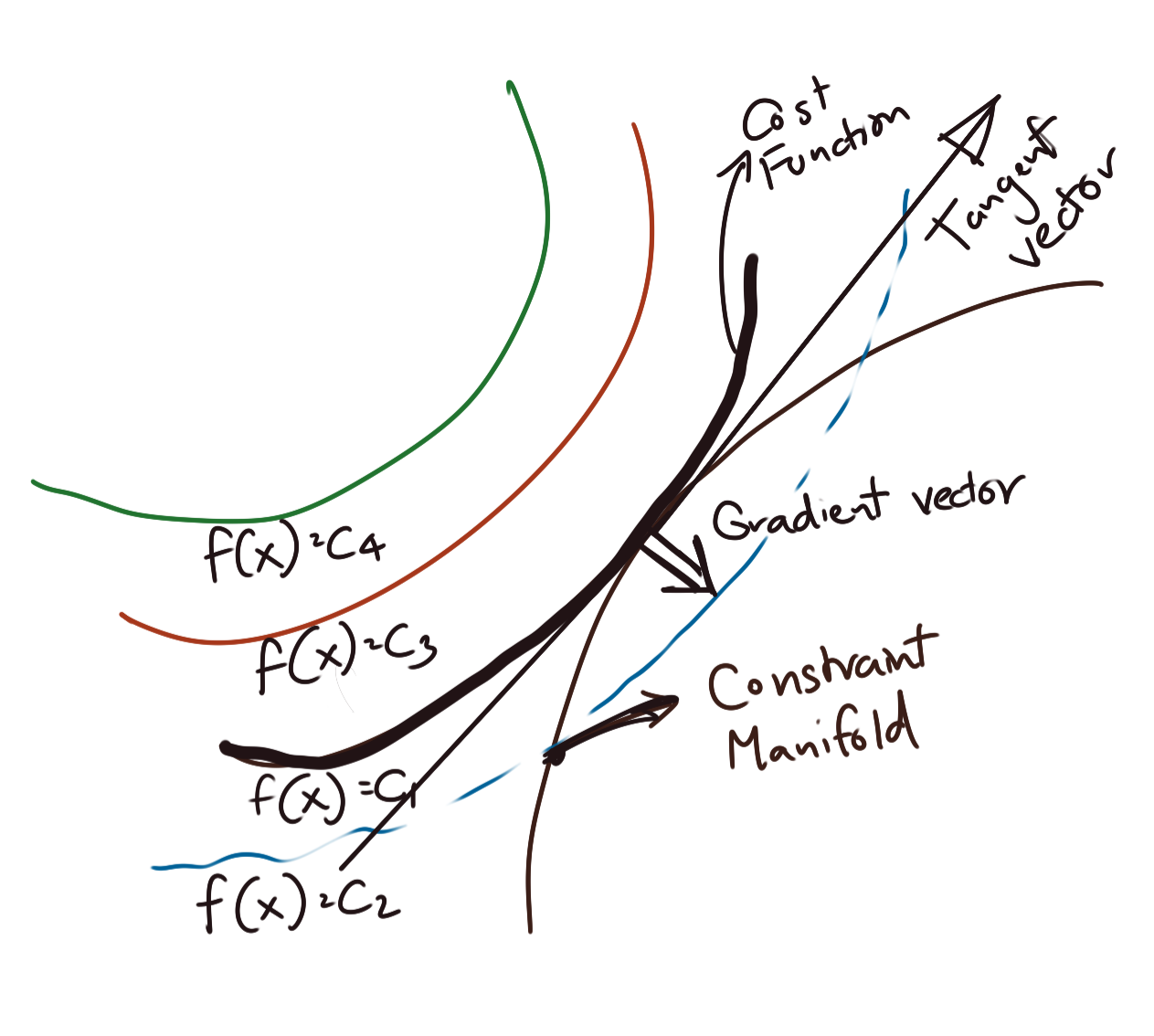
Now, usually when we attempt to find the optimum point on a function (in this case, say \(f(U,V)\)), we would want to take its derivative and set it to zero. However, in the presence of other constraints, the point that we seek is not necessarily the global maximum/minimum, since that point (or those points) are not necessarily guaranteed to satisfy the constraints simultaneously. We still want a maximum/minimum, but we also want it to live on the constraint manifold. What we can say is that the direction derivative of the function \(f(U,V)\) in the direction of any vector in its tangent space will go to zero.

Restated another way, the gradient normal vector of the function \(F(U,V)\) is orthogonal to every vector in the tangent space of \(F(U,V)\). Since orthogonality implies a dot product of zero, given the constraints we have, we can write the following condition as necessary for finding a critical point:

\[\mathbf{ D_{(U,V)}f=\nabla f.T_X=0 }\]

where:

• \(\mathbf{\nabla f}\) is \(\mathbf{1 \times (m+n)}\)
• \(\mathbf{T_X}\) is \(\mathbf{(m+n)\times m}\)
• \(\mathbf{D_{(U,V)}f}\) is \(\mathbf{1 \times m}\).

The figure below shows a simplified situation.

Proof of Lagrange Multipliers

We are about three-quarters of the way done. We have proved that the tangent space belongs to the kernel (null space) of the gradient vector. But we haven’t gotten to proving the assertion about Lagrange Multipliers yet. What we really need to prove is that the gradient vector can be expressed as linear combinations of the vectors in tangent space, which will lead us directly to the conclusion we are hoping to prove.

We need to express another identity, using the level sets of the original constraint functions themselves. If you remember, \(G\) has been derived through row reduction techniques from the original \(n\) constraint functions. Let’s call them \(h_i\), and define them as below:

\[h_1(u_1,u_2,u_3,...,u_m,v_1,v_2,v_3,...,v_n)=c_1 \\ h_2(u_1,u_2,u_3,...,u_m,v_1,v_2,v_3,...,v_n)=c_2 \\ h_3(u_1,u_2,u_3,...,u_m,v_1,v_2,v_3,...,v_n)=c_3 \\ \vdots \\ h_n(u_1,u_2,u_3,...,u_m,v_1,v_2,v_3,...,v_n)=c_n\]

More generally, we write: \(h_i(U,V)=c_i\)

Taking the derivative, and remembering that \(U=(u_1, u_2, u_3,...,u_m)\), \(V=(v_1, v_2, v_3,...,v_m)\) are shorthands for the reams of variables that I’d like to not write:

\[\frac{\partial h_i(U,V)}{\partial U}=0 \\ \Rightarrow \frac{\partial h_i(U,V)}{\partial (U,V)}.\frac{\partial G(U)}{\partial U}=0 \\ \Rightarrow \mathbf{D_{(U,V)h_i}.T_X=0}\]

If we define:

\[H=\begin{bmatrix} h_1 \\ h_2 \\ \vdots \\ h_n \\ \end{bmatrix}\]

We can write:

\[\mathbf{D_{(U,V)}H.T_X=0}\]

Do check that the indexes match: \(H\) is \(m \times (m+n)\), and \(T_X\) is \((m+n) \times m\), so yes, they are compatible.

We now have these two identities:

\[\mathbf{ D_{(U,V)}f.T_X=\nabla f.T_X=0 \\ D_{(U,V)}H.T_X=0 }\]

Let’s get rid of some extraneous notation to get:

\[\mathbf{ Df.T_X=0 \\ DH.T_X=0 }\]

This implies that:

\[C(T_X) \subset N(Df) = {R(Df)}^{\perp}\\ C(T_X) \subset N(DH) = {R(DH)}^{\perp}\]

Let us make some observations on the ranks of these matrices:

• \(T_X\) is \((m+n) \times m\), but has rank \(m\). \(f\) is \(1\times (m+n)\). \(f\) can have at most rank 1.
• \(T_X\) is \((m+n) \times m\), but has rank \(m\). \(H\) is \(n \times (m+n)\), so its maximum column/row rank is \(n\). Then, by the Rank-Nullity Theorem, its left null space/null space has rank \(m\).

\(C(T_X)\) and \({R(DH)}^{\perp}\) have the same rank \(m\). Thus they are equal. This implies that:

\[{R(DH)}^{\perp} \subset {R(Df)}^{\perp}\]

By the Subset Rule, we can say:

\[{({R(DH)}^{\perp})}^{\perp} \supset {({R(Df)}^{\perp})}^{\perp} \\ \Rightarrow R(DH) \supset R(Df)\]

Check the indexes again:

• \(DH\) is \(n \times (m+n)\), so \(n\) row vectors of length \((m+n)\) each.
• \(Df\) is \(1 \times (m+n)\), so 1 row vector of length \((m+n)\).

This implies that the row span of \(Df\) is contained within the row span of \(DH\). To put it another way:

The row vector of \(Df\) can be expressed as a linear combination of the row vectors of \(DH\).

Thus, we can write:

\[\mathbf{ Df=\lambda_1 Dh_1(U,V)+\lambda_2 Dh_2(U,V)+\lambda_3 Dh_3(U,V)+...+\lambda_n Dh_n(U,V) } \\ \square\]

The weights of these linear combinations are called Lagrange Multipliers. We can simplify this notationally to:

\[\mathbf{ \nabla f={[\nabla H]}^T\lambda }\]

where:

• \(\nabla f\) is \((m+n) \times 1\) (1 function, partial derivatives in \(m+n\) variables)
• \(\nabla H\) is \(n \times (m+n)\) (\(n\) equations, partial derivatives in \(m+n\) variables)
• \(\lambda\) is \(n\times 1\) (\(n\) Lagrange multipliers)

Generalisation to Nonlinear Functions

There is an important assumption I’ve left unsaid. In every example we’ve seen, I’ve always said that the constraints represent a system of linear equations. This might be true if our constraint equations are always straight lines, but is certainly not the case in other situations. Some examples of nonlinear constraints are:

• \[x^2+x^3+y=3\]
• \[xy+z=4\]
• \[xy^4+z=4\]

In all but a few “easy” cases, it is absolutely not possible to factor out variables, such that some dependent variables are expressed in terms of some independent variables. Even if that were possible, the assumption of a linear relationship would not hold.

That is not the only problem. Constraint equations define the solution space such that even if the constraints are individually tractable to analyse, the manifold formed by their intersection cannot be described by any easily-discovered equation, linear or non-linear.

For example, take a look at this beauty.

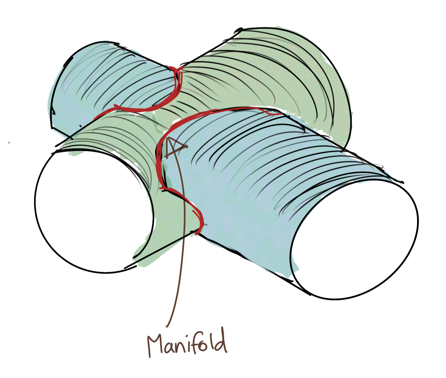
The red line shows the manifold, which satisfies the equations of both these cylinders. This intersection is not easily expressible; also it is guaranteed to be nonlinear in nature. And this is just two cylinders. It is not uncommon to have more constraint equations, all similarly nonlinear, and possibly higher-dimensional. We cannot even visualise such surfaces, let alone the intersections between them.

How are we to resolve this quandary?

Implicit Function Theorem

Functions come in many shapes and sizes. They aren’t always necessarily linear. However, that does not mean that analysis of these nonlinear functions is intractable. Calculus makes the mostly nonlinear world around us, and tells us that we can treat any curve or surface, in any dimension, as linear if we only zoom into it close enough.

It basically asks us to pretend that a complicated curve (and the corresponding function) is a linear function. This approximation is grossly wrong at larger scales, but gets better and better the more we zoom in. This is essentially the concept behind tangents to curves. The slope of a tangent comes from considering two points: one point on the curve proper, and another curve in the neighbourhood of the first point, which is as close as possible to the first point, but not the same as the first point.

In calculus, this is termed the limit. That \(\frac{dy}{dx}\) that we bandy about so much, essentially expresses a linear relationship between \(x\) and \(y\) at that point. This piecewise linearity at infinitesmal scales is what enables us to frame problems in a way that are solvable, instead of being overwhelmed by the nonlinearity of the function.

In practice, we speak of locality: the neighbourhood of a point, as being a small non-zero-sized area around the point, smaller than you can possibly imagine. Then, you carry out your nice linear calculations in this neighbourhood, assured of the fact that you have zoomed in enough that the function looks linear.

Let us return to our original quandry: how can we even begin to find a critical point on a constraint manifold if we do not even know how to express some variables in terms of others in the constraint equations? Remember, this parameterisation is what allows us to encode the constraints of the manifold into the function of the curve that we desire to find a critical point on.

The first question we ask is: does such a relationship even exist? And since this is calculus, we ask whether this relationship exists locally, i.e., when we zoom in. Even if we only know whether it exists locally, that can still help us discover useful properties about the curve. The third question we can ask is whether we can know any aspects of this relationship.

The Implicit Function Theorem has an answer to these questions.

We will not delve much into the Implicit Function Theorem, merely state its results. That itself should validate the assumption around the linear relationship that we have been using all this time.

The Implicit Function Theorem states that if a mapping \(F(x)\) exists for a point \(c\) such that:

• \[\mathbf{F(c)=0}\]
• \(F(c)\) is first order differentiable (\(C^1\) differentiable)
• The derivative of F(c), i.e., \(DF(c)\) is onto, i.e., for every value of \(DF(c)\), there exists a corresponding input.

then, the following holds true:

• There exists a system of linear equations \(DF(c)=0\) which has \(n\) pivotal variables in the level set constraint equations which can be expressed as functions of \(m\) independent (non-pivotal) variables.
• There is a neighbourhood of \(c\) where this linear relationship holds for \(F(c)=0\).

We could not have made the assumption of the existence of this mapping and its inverse for the general case of nonlinear constraints without the Implicit Function Theorem.

---