Quadratic Optimisation using Principal Component Analysis as Motivation: Part Two

Avishek Sen Gupta on 28 April 2021

---

We pick up from where we left off in Quadratic Optimisation using Principal Component Analysis as Motivation: Part One. We treated Principal Component Analysis as an optimisation, and took a detour to build our geometric intuition behind Lagrange Multipliers, wading through its proof to some level.

We now have all the machinery we need to tackle the PCA problem directly. As we will see, the Lagrangian approach to optimisation maps to this problem very naturally. It will probably turn out to be slightly anti-climactic, because the concept of eigenvalues will fall out of this application quite naturally.

Eigenvalues and Eigenvalues

We glossed over Eigenvalues and Eigenvectors when we looked at PCA earlier. Any basic linear algebra text should be able to provide you the geometric intuition of what an eigenvector of a matrix \(A\) is, functionally.

If we consider the matrix \(A\) as a \(n \times n\) matrix which represents a mapping \(\mathbb{R}^n \rightarrow \mathbb{R}^n\) which transforms a vector \(\vec{v} \in \mathbb{R}^n\), then \(\vec{v}\) is an eigenvector of \(A\) if the following condition is satisified:

\[\mathbf{A\vec{v}=\lambda\vec{v}, \lambda \in \mathbb{R}}\]

That is, regardless of what effect \(A\) has on other vectors (which are not collinear with \(\vec{v}\)) transforming vector \(\vec{v}\) results in only a scaling of \(\vec{v}\) by a real number \(\lambda\). \(\lambda\) is called the corresponding eigenvalue of \(A\).

There can be multiple eigenvalue/eigenvector values for a matrix. For the purposes of this article, it suffices to state that Principal Components Analysis is one of the methods of determining these components of a matrix.

Well, let’s rephrase that. Since PCA works on the covariance matrix, the eigenvectors and eigenvalues are those of the covariance matrix, not the original matrix. However, that does not affect what we are aiming for, which is finding the principal axes of maximum variance.

Lagrange Multipliers are Eigenvalues

Let us pick up the optimisation problem where we left off:

Maximise \(X^T\Sigma X\)
Subject to: \(X^TX=1\)

We spoke of quadratic forms as well; this is clearly a quadratic form of the matrix \(\Sigma\). Armed with our knowledge of vector calculus, let us state the above problem in terms of geometry.

Find the critical point \(X\) on \(f(X)=X^T\Sigma X:\mathbb{R}^n\rightarrow \mathbb{R}\) such that:

• \(X\) lies on the unit sphere, i.e., the manifold equation is \(\mathbf{g(X)=X^TX=1}\).

This is what the solution space might look like in the two-dimensinal case.

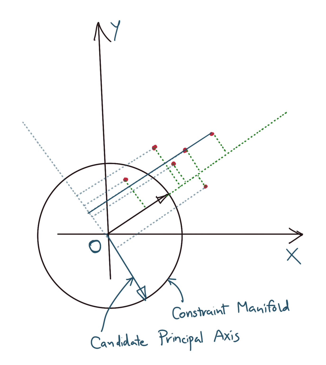
Let \(g(x)\) be the constraint manifold. We now wish to compute the derivatives of the cost function of \(f(X)\) and the manifold equation \(g(x)\).

For the cost function \(f(X)\), so we can write:

\[D_Xf(X)=D[X^T\Sigma X] \\ = X^T\Sigma+X^T\Sigma^T \\ =X^T(\Sigma+{\Sigma}^T) \\ =2X^T\Sigma \text{ (since } \sigma \text{ is symmetric, } \Sigma=\Sigma^T \text{)}\]

Taking the derivative of the manifold equation \(g(x)\), we get:

\[D_Xg(X)=2X^T\]

The Lagrange approach tells us that there exists a Lagrange Multiplier \(\lambda_1\) for which the following holds true:

\[D_Xg(X)=\lambda_1 D_Xf(X) \\ \Rightarrow 2X^T\Sigma=\lambda_1 2X^T \\ \Rightarrow X^T\Sigma=\lambda_1 X^T\]

Taking the transpose on both sides, we get:

\[{(X^T\Sigma)}^T={(\lambda_1 X^T)}^T \\ \Rightarrow \mathbf{\Sigma^T X=\lambda_1 X}\]

That’s right, eigenvalues are nothing but Lagrange Multipliers when optimising for Principal Components Analysis!

We can go further, assuming there is more than one eigenvalue / eigenvector pair for matrix \(\Sigma\). Let us assume that \(\Sigma\) has two eigenvalues / eigenvectors. Let \(X_1\) be the first one, which we have already found. \(X_2\) is the second eigenvector. The necessary conditions for this eigenvector to exist are:

• \({X_2}^T{X_2}=1\), i.e., \(X_2\) exists on the constraint manifold of a unit circle.
• \(X_2.X_1=0\), i.e., \(X_2\) is orthogonal to \(X_1\)

The same argument as the first part of the proof holds, that is:

\[D_Xf(X)=\mu X_1+\lambda_2 X_2 \\ \Sigma X_2=\mu X_1+\lambda_2 X_2 \\\]

We have put in \(\mu\) as the multiplier for \(X_1\) because we do not know what value will be, that is, we need to determine its value. Take the dot product with \(X_1\) on both sides, so we can write:

\[(\Sigma X_2).X_1=\mu X_1.X_1+\lambda_2 X_2.X_1\]

Dot products are commutative, and we know that X_1.X_0=0, thus we write:

\[(\Sigma X_2).X_1=\mu X_1.X_1+\lambda_2 X_2.X_1 \\ \Rightarrow \mu X_1.X_1=0 \\ \Rightarrow \mu {\|X_1\|}^2=0 \\ \Rightarrow \mu=0\]

Substituting \(\mu=0\) back into the original Lagrange Multipliers equation, we get:

\[\mathbf{ \Sigma X_2=\lambda_2 X_2 }\]

You can repeat this proof for every eigenvector.

Spectral Theorem of Matrices

You may not realise it, but we have also proved an important theorem of Linear Algebra, namely, the Spectral Theorem of Matrices, in this case, for symmetric matrices. It states a few things, two of which we have already proved.

• \[\mathbf{A\vec{v}=\lambda\vec{v}}: \lambda \in \mathbb{R}, \vec{v} \in \mathbb{R}^n, A^T=A, A \in \mathbb{R}^n \times \mathbb{R}^n\]
• For every symmetric matrix \(A\), there exists a decomposition \(UDU^T\), where the columns of \(U\) are the eigenvectors of \(A\), and \(D\) is a diagonal matrix whose diagonal entries are the corresponding eigenvalues.
• For non-symmetric matrices, the factorisation \(A=UDU^{-1}\) still exists.

To see why the second statement is true, write out \(U\) and \(D\) as:

\[U=\begin{bmatrix} \vert && \vert && \vert && ... && \vert \\ v_1 && v_2 && v_3 && ... && v_n \\ \vert && \vert && \vert && ... && \vert \end{bmatrix} \\ \\ D==\begin{bmatrix} \lambda_1 && 0 && 0 && ... && 0 \\ 0 && \lambda_2 && 0 && ... && 0 \\ 0 && 0 && \lambda_3 && ... && 0 \\ \vert && \vert && \vert && ... && \vert \\ 0 && 0 && 0 && ... && \lambda_n \\ \end{bmatrix}\]

Then, if we multiply them, we get:

\[UD=\begin{bmatrix} \vert && \vert && \vert && ... && \vert \\ \lambda_1 v_1 && \lambda_2 v_2 && \lambda_3 v_3 && ... && \lambda_3 v_n \\ \vert && \vert && \vert && ... && \vert \end{bmatrix} \\ =\begin{bmatrix} \vert && \vert && \vert && ... && \vert \\ A v_1 && A v_2 && A v_3 && ... && A v_n \\ \vert && \vert && \vert && ... && \vert \end{bmatrix} \\ = AU\]

Thus, we have the identity: \(AU=UD\). Multiplying both sides by \(U^{-1}\), and remembering that for orthonormal matrices, \(X^{-1}=X^T\), we get:

\[AUU^{-1}=UDU^{-1} \Rightarrow AI=UDU^T \Rightarrow \mathbf{A=UDU^T}\]

This proves that for every symmetric matrix \(A\), there exists a decomposition \(UDU^T\), where the columns of \(U\) are the eigenvectors of \(A\), and \(D\) is a diagonal matrix, whose diagonal entries are the corresponding eigenvalues of \(A\).

We have established a deep connectin between Lagrange Multipliers and eigenvalues of a matrix. However, Quadratic Programming covers some more material, which will be relevant when completing the derivation of the Support Vector Machine equations. This will be covered in an upcoming post.

Supplementary Material

1. Proof that \(X^{-1}=X^T\) for orthonormal matrices

Quick Note: Orthogonal and Orthonormal mean the same thing.

Suppose \(X\) is an orthonormal matrix like so:

\[U=\begin{bmatrix} \vert && \vert && \vert && ... && \vert \\ x_1 && x_2 && x_3 && ... && x_n \\ \vert && \vert && \vert && ... && \vert \end{bmatrix} \\ U^T=\begin{bmatrix} --- && x_1 && --- \\ --- && x_2 && --- \\ --- && x_3 && --- \\ \hspace{2cm} && \vdots && \hspace{2cm} \\ --- && x_n && --- \\ \end{bmatrix}\]

Then, multiplying the two, the following identity holds:

\[A_{ij}=0, i\neq j \\ A_{ij}=1, i=j (orthonormality)\] \[U^TU=I=U^{-1}U \\ \Rightarrow U^TU=U^{-1}U \\ \Rightarrow \mathbf{U^T=U^{-1}}\]

---