Geometry of the Multivariate Gaussian Distribution

Avishek Sen Gupta on 30 August 2021

---

Continuing from the roadmap set out in Road to Gaussian Processes, we begin with the geometry of the central object which underlies this Machine Learning Technique, the Multivariate Gaussian Distribution. We will study its form to build up some geometric intuition around its interpretation.

To do this, we will cover the following preliminaries.

• Algebraic form of the \(n\)-dimensional ellipsoid
• Projection as Change of Basis

Algebraic form of the \(n\)-dimensional ellipsoid

The standard form of an ellipsoid in \(\mathbb{R}^2\) is:

\[\frac{ {(x-x_0)}^2}{a^2} + \frac{ {(y-y_0)}^2}{b^2}=C\]

Generally, for an \(n\)-dimensional ellipsoid, the standard form is:

\[\sum_{i=1}^n \frac{ {(x_i-\mu_i)}^2}{\lambda_i^2}=C\]

Let us denote \(X=\begin{bmatrix}x_1\\x_2\\ \vdots\\ x_n\end{bmatrix}\), \(\mu=\begin{bmatrix}\mu_1\\\mu_2\\ \vdots\\ \mu_n\end{bmatrix}\) and

\[D=\begin{bmatrix} \lambda_1 && 0 && 0 && \cdots && 0 \\ 0 && \lambda_2 && 0 && \cdots && 0 \\ 0 && 0 && \lambda_3 && \cdots && 0 \\ \vdots && \vdots && \vdots && \ddots && \vdots \\ 0 && 0 && 0 && \cdots && \lambda_n \\ \end{bmatrix}\]

Then, we can see that:

\[\begin{equation} D^{-1}=\begin{bmatrix} \frac{1}{\lambda_1} && 0 && 0 && \cdots && 0 \\ 0 && \frac{1}{\lambda_2} && 0 && \cdots && 0 \\ 0 && 0 && \frac{1}{\lambda_3} && \cdots && 0 \\ \vdots && \vdots && \vdots && \ddots && \vdots \\ 0 && 0 && 0 && \cdots && \frac{1}{\lambda_n} \\ \end{bmatrix} \label{eq:diagonal} \end{equation}\]

Then, we can rewrite the standard form of the \(n\)-dimensional ellipsoid as:

\[{\|D^{-1}(X-\mu)\|}^2=C \\\]

Alternatively, we can write:

\[\begin{equation} \mathbf{ {[D^{-1}(X-\mu)]}^T [D^{-1}(X-\mu)]=C } \label{eq:algebraic_n_ellipsoid} \end{equation}\]

This can be easily verified by expanding out the terms. like so:

\[D^{-1}(X-\mu)=\begin{bmatrix} \frac{1}{\lambda_1} && 0 && 0 && \cdots && 0 \\ 0 && \frac{1}{\lambda_2} && 0 && \cdots && 0 \\ 0 && 0 && \frac{1}{\lambda_3} && \cdots && 0 \\ \vdots && \vdots && \vdots && \ddots && \vdots \\ 0 && 0 && 0 && \cdots && \frac{1}{\lambda_n} \\ \end{bmatrix} \bullet \begin{bmatrix}x_1-\mu_1\\x_2-\mu_2\\ \vdots\\ x_n-\mu_n\end{bmatrix} = \begin{bmatrix}\frac{x_1-\mu_1}{\lambda_1}\\\frac{x_2-\mu_2}{\lambda_2}\\ \vdots\\ \frac{x_n-\mu_n}{\lambda_n}\end{bmatrix}\]

Then, expanding out \(\eqref{eq:algebraic_n_ellipsoid}\), we get:

\[{[D^{-1}(X-\mu)]}^T [D^{-1}(X-\mu)]=C \\ \Rightarrow \begin{bmatrix}\frac{x_1-\mu_1}{\lambda_1} && \frac{x_2-\mu_2}{\lambda_2} && \cdots && \frac{x_n-\mu_n}{\lambda_n}\end{bmatrix} \bullet \begin{bmatrix}\frac{x_1-\mu_1}{\lambda_1}\\\frac{x_2-\mu_2}{\lambda_2}\\ \vdots\\ \frac{x_n-\mu_n}{\lambda_n}\end{bmatrix}\\ = \sum_{i=1}^n \frac{ {(x_i-\mu_i)}^2}{\lambda_i^2}=C\]

Projection as Change of Basis for an Orthonormal Basis

We have already discussed projections of vectors onto other vectors in several places (for example, in Gram-Schmidt Orthogonalisation). We can look at vector projection through a different lens, namely as a change in coordinate system.

Consider a vector \(B\) in the standard basis of \(\mathbb{R}^2\). We know that the standard basis of \(\mathbb{R}^2\) is only one of an infinite number of bases we can use. Let us pick another orthogonal basis \(X`\) and \(Y'\). They have to be linearly independent. Furthermore, we assume that they are unit vectors, i.e., \(\|X`\|=\|Y`\|=1\).

Then, the projection coefficient of \(B\) onto \(X`\) and \(Y`\) are:

\[\text{proj}_{BX'}=\frac{ {X'}^T B}{ {X'}^T X'}={X'}^T B \text{ (since X' is a unit vector)} \\ \text{proj}_{BY'}=\frac{ {Y'}^T B}{ {Y'}^T Y'}={Y'}^T B \text{ (since Y' is a unit vector)}\]

The situation is as shown below.

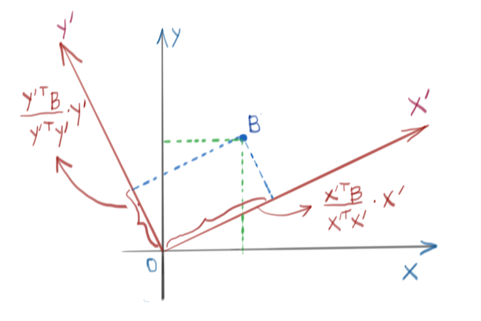
These projection coefficients are the coordinates of \(B\) in the new coordinate system defined by \(X'\) and \(Y'\). To recover \(B\), you can simply multiply out the projections by respective basis vectors \(X'\) and \(Y'\).

More generally, for any new basis matrix \(C\) (assuming the basis vectors are unit vectors), any vector \(V\) can be written as:

\[V_C=C^TV\]

Analogous to the above example, we can recover the original vector \(V\) by writing \(V=C^TVC\).

Notes: Change of Basis for a Non-Orthogonal Basis

The reason we chose an orthonormal basis for our illustration is because a change of basis of a non-orthogonal basis cannot be represented by a vertical projection. The situation with a non-orthogonal basis is shown below.

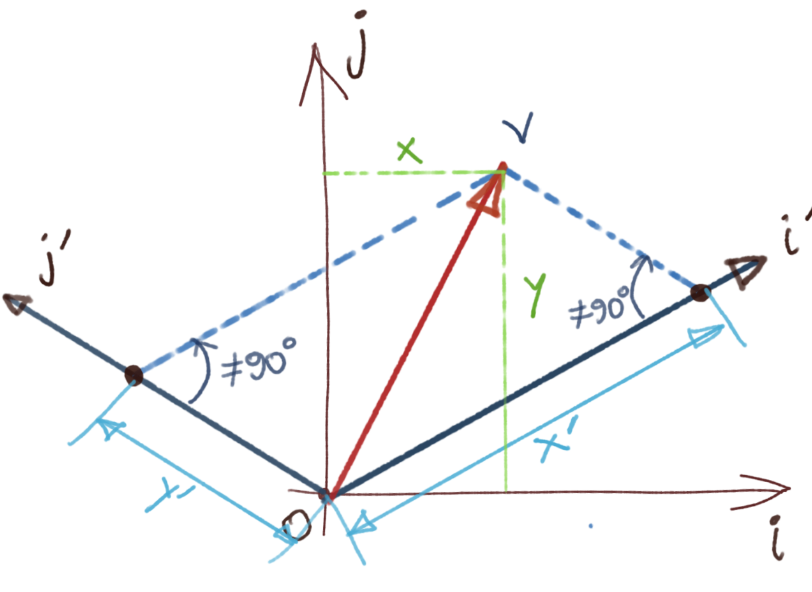
In that case, we use the identity:

\[B_1 v_1=B_2 v_2\]

In the case of \(B_1\) being the standard basis (identity matrix), we get:

\[B_2 v_2=v_1 \\ \Rightarrow v_2={B_2}^{-1} v_1\]

You should notice that since in the special orthogonal case we discussed above, \({B_2}^{-1}={B_2}^T\), and the above identity reduces to the vertical projection case we talked about above.

Geometry of the Tilted Ellipsoid

Assume an arbitrary point \(X\) in \(\mathbb{R}^n\). Let us choose a different basis \(C\). Then, \(X_C=C^TX\). An ellipsoid in this new coordinate system (centered at the origin) is then given by:

\[{[D^{-1}X_C]}^T [D^{-1}X_C]=K \\ \Rightarrow {[D^{-1}C^TX]}^T [D^{-1}C^TX]=K\]

where \(D^{-1}\) was already defined as in \(\eqref{eq:diagonal}\), and \(K\) is a constant. If the ellipsoid was centered at \(\mu\), then the above expression becomes:

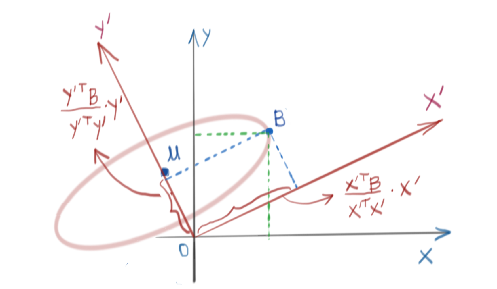
\[\begin{equation} {[D^{-1}C^T(X-\mu)]}^T [D^{-1}C^T(X-\mu)]=K \label{eq:tilted-ellipsoid} \end{equation}\]

The situation in \(\mathbb{R}^2\) is shown below.

Multivariate Gaussian Distribution

We are now in a position to understand the form of the Multivariate Gaussian Distribution. The standard form of the Multivariate Gaussian Distribution is given by:

\[\mathbf{ G(X)=C\bullet\exp\left( -\frac{1}{2} {(X-\mu)}^T\Sigma^{-1}(X-\mu) \right) }\]

where \(\Sigma\) is the (invertible) covariance matrix. Let us note some specific properties of the covariance matrix before proceeding further.

• The covariance matrix can be diagonalised.
• The covariance matrix is symmetric. This implies that all its eigenvectors are orthogonal.

We seek to understand the shape of this Gaussian. To do that, let us fix the value of \(G(X)\) to, say, \(K\).

\[C\bullet \exp\left(-\frac{1}{2} {(X-\mu)}^T \Sigma^{-1} (X-\mu)\right)=K\]

Let us express \(\Sigma^{-1}\) in terms of its eigenvectors.

\[\Sigma=VDV^{-1}=VDV^T \\ \Sigma^{-1}={(VDV^T)}^{-1} \\ \Sigma^{-1}=V^{-T}D^{-1}V^{-1}=VD^{-1}V^T \\ \mathbf{\Sigma^{-1}=VD^{-1}V^T}\]

Substituting this result into the original expression, we get:

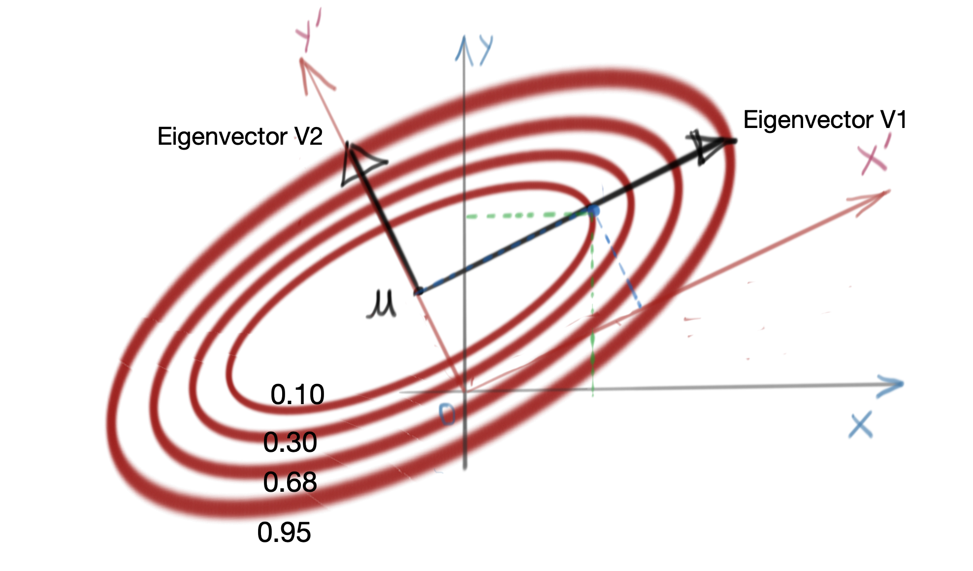
\[C\bullet \exp\left(-\frac{1}{2}{(X-\mu)}^T VD^{-1}V^T (X-\mu)\right)=K \\ \exp\left(-\frac{1}{2}{(X-\mu)}^T VD^{-\frac{1}{2}} D^{-\frac{1}{2}} V^T (X-\mu)\right) = \frac{K}{C}\] \[\begin{equation} \mathbf{ {[D^{-\frac{1}{2}} V^T (X-\mu)]}^T [D^{-\frac{1}{2}} V^T (X-\mu)] = -2\text{ ln}\frac{K}{C} = K_0 } \label{eq:constant-probability-ellipse} \end{equation}\]

The above expression corresponds directly to the form of a tilted ellipsoid in \(\eqref{eq:tilted-ellipsoid}\). This implies that the contour of constant probability of a Multivariate Gaussian Distribution is a tilted ellipsoid.

The basis for this tilt, i.e., the coordinate system used is the set of eigenvectors of the covariance matrix \(\Sigma\).

For example, in \(\mathbb{R}^2\), the major and minor axes of the ellipse are oriented in the directions of the eigenvectors, as shown below.

Special Case: Independent Random Variables

If the random variables in a Multivariate Gaussian Distribution are independent, then the covariance matrix is essentially a diagonal matrix, and its eigenvectors form the standard basis in \(\mathbb{R}^n\). Thus, the eigenvector matrix becomes the identity matrix. This implies that there is effectively no change in the basis, and the ellipsoids of constant probability are not tilted, and the form in \(\eqref{eq:constant-probability-ellipse}\) becomes:

\[\mathbf{ {[D^{-\frac{1}{2}} (X-\mu)]}^T [D^{-\frac{1}{2}} (X-\mu)] = K_0 }\]

---