Common Ways of Looking at Matrix Multiplications

Avishek Sen Gupta on 29 April 2021

---

We consider the more frequently utilised viewpoints of matrix multiplication, and relate it to one or more applications where using a certain viewpoint is more useful. These are the viewpoints we will consider.

• Linear Combination of Columns
• Linear Combination of Rows
• Linear Transformation
• Sum of Columns into Rows
• Dot Product of Rows and Columns
• Block Matrix Multiplication

Linear Combination of Columns

This is the most common, and probably one of the most useful, ways of looking at matrix multiplication. This is because the concept of linear combinations of columns is a fundamental way of determining linear independence (or linear dependence), which then informs us about many things, including:

• Dimensionality of the column space and row space
• Dimensionality of the null space and left null space
• Uniqueness of solutions
• Invertibility of matrix

This is obviously the most commonly used interpretation when defining and working with vector subspaces, as well.

Linear Combination of Rows

There’s not much more to say about the linear combinations of rows. However, any deduction about the row rank of a matrix from looking at its row vectors automatically applies to the column rank as well, so it is useful in situations where you find looking at rows easier than columns.

Sum of Columns into Rows

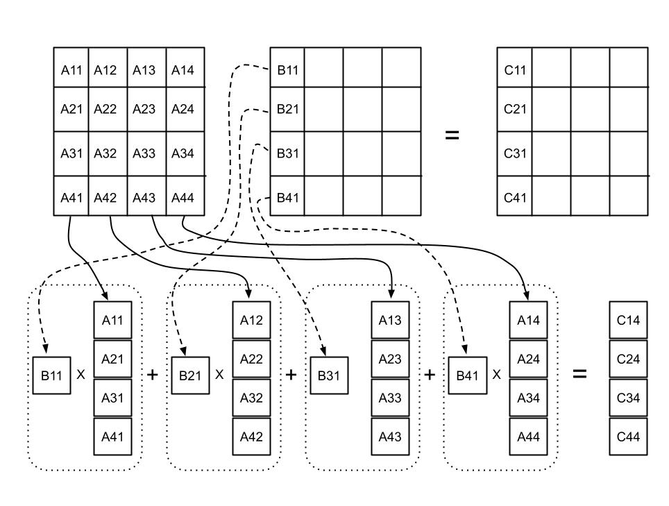
The product of a column of the left matrix and a row of the right matrix gives a matrix of the same dimensions as the final result. Thus, each product results in one “layer” of the final result. Subsequent “layers” are added on through summation. Thus, product looks like so:

Thus, for \(A\in\mathbb{R}^{m\times n}\) and \(B\in\mathbb{R}^{n\times p}\), we can write out the multiplication operation as below:

\[\mathbf{AB=C_{A1}R_{B1}+C_{A2}R_{B2}+C_{A3}R_{B3}+...+C_{An}R_{Bn}}\]

This is a common form of treating a matrix when performing LU Decomposition. See Matrix Outer Product: Columns-into-Rows and the LU Factorisation for an extended explanation of the LU Factorisation.

Linear Transformation

This is a very common way of perceiving matrix multiplication in computer graphics, as well as when considering change of basis. Lack of matrix invertibility can also be explained through whether a vector exists which can can be transformed into the zero vector by said matrix.

Dot Product of Rows and Columns

This is the common form of treating matrices when doing proofs where the transpose invariance property of symmetric matrices is utilised, i.e., \(A^T=A\). It is also the one taught in high school the most, and not really the best way to start understanding matrix multiplication.

Block Matrix Multiplication

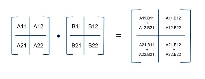
The block matrix multiplication is not really a separate method of multiplication per se. It is more of a method for bringing a higher level of abstraction in a matrix, while still permitting the “blocks” to be treated as singular matrix entries.

One application of this is when proofs involve properties of a larger matrix composed of submatrices, which have interesting properties of their own, which we wish to exploit.

An interesting example is part of the statement of the Implicit Function Theorem. In one dimension, the validity of this theorem holds when the function being described is monotonic in a defined interval (always increasing or always decreasing in that interval). In higher dimensions, this requirement of monotonicity is stated more formally as saying that the derivative of the function is invertible within a defined interval. We discussed this theorem in the article on Lagrange Multipliers.

The motivation for this example is the mathematical description of that monotonicity requirement. More on this is discussed in Intuitions about the Implicit Function Theorem.

We can prove that a matrix which looks like this:

\[X= \begin{bmatrix} A && C \\ 0 && B \end{bmatrix}\]

where \(A\), \(B\) are invertible submatrices, and \(I\) is the identity matrix, the matrix \(X\) is also invertible. Let us be precise about the dimensions of these matrices.

\[X=(n+m)\times (n+m) \\ A=n \times n \\ 0=m \times n \\ C=n \times m \\ B=m \times m\]

Do verify for yourself that these submatrices align. To prove this, let us assume there exists a matrix \(X^{-1}\), which is the inverse of \(X\). Therefore, \(XX^{-1}=I\). Furthermore, let us assume the form of \(X^{-1}\) to be:

\[X^{-1}=\begin{bmatrix} P && Q \\ R && S \end{bmatrix}\]

Again, we make precise the dimensions of the submatrices of \(X^{-1}\).

\[P=n \times n \\ Q=n \times m \\ R=m \times n \\ S=m \times m\]

If we multiply \(XX^{-1}\), we get:

\[XX^{-1}= \begin{bmatrix} AP+CR && AQ+CS \\ BR && BS \end{bmatrix}= \begin{bmatrix} I_{n \times n} && 0_{n \times m} \\ 0_{m \times n} && I_{m \times m} \end{bmatrix}\]

Let’s do a quick sanity check. Checking back to the dimensions of the matrices, we can immediately see that:

-\(AP\) and \(CR\) give a \(n \times n\) matrix. -\(BS\) gives a \(m \times m\) matrix. -\(AQ\) and \(CS\) give a \(n \times m\) matrix. -\(BR\) give a \(m \times n\) matrix.

The cool thing is that you can write out the element-wise equalities, and solve for \(P\), \(Q\), \(R\), \(S\), as if they were simple variables, as long as you adhere to the matrix operation rules of ordering, transpose, inverse, etc.

Thus, we can write:

\[AP+CR=I \\ AQ+CS=0 \\ BR=0 \\ BS=I\]

From the last two identities, we can immediately say that:

\[R=0 \\ S=B^{-1}\]

Solving for the remaining two variables \(P\) and \(Q\), we get:

\[P=A^{-1} \\ Q=-A^{-1}CB^{-1}\]

Thus the inverse of \(X\) is:

\[XX^{-1}= \begin{bmatrix} A^{-1} && A^{-1}CB^{-1} \\ 0 && B^{-1} \end{bmatrix}\]

The important point to note here is that the solution does not need \(C\) to be an invertible matrix; it may be rank-deficient, and \(X\) still remains an invertible matrix.

Recursive Calculation

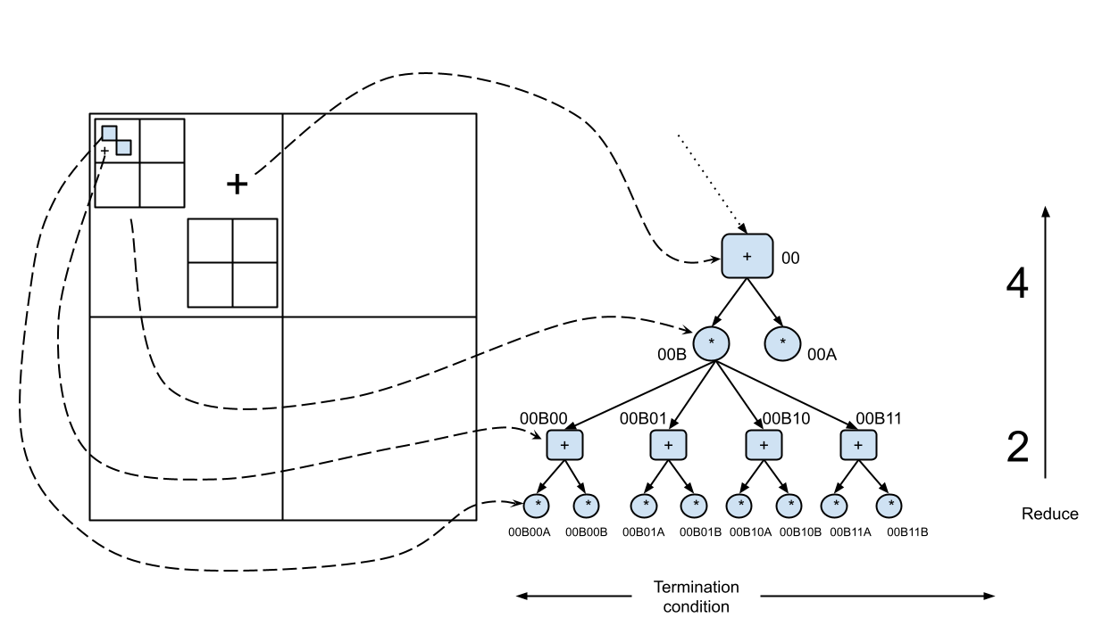
The block matrix calculation can be extended to be recursive. We can simply break down any submatrix into its block matrices and perform the same operation, until (if you so wish) you reach the individual element level.

---