We discussed the Implicit Function Theorem at the end of the article on Lagrange Multipliers, with some hand-waving to justify the linear behaviour on manifolds in arbitrary \(\mathbb{R}^N\).
This article delves a little deeper to develop some more intuition on the Implicit Function Theorem, but starts with its more specialised relative, the Inverse Function Theorem. This is because it is easier to start with reasoning about the Inverse Function Theorem.
Inverse Functions
Monotonicity in One Dimension
Let’s start with a simple motivating example. We have the function \(f(x)=2x: x \in \mathbb{R}^n\). This gives a value, say \(y\), given an \(x\). We desire to find a function \(f^{-1}\) which is the inverse of \(f^{-1}\), i.e., given a \(y\), we wish to recover \(x\). Mathematically, we can say:
\[f^{-1}(f(x))=x\]In this case, the inverse is pretty easy to determine, it is \(f^{-1}(x)=\frac{x}{2}\). The function \(f\) is thus a mapping from \(\mathbb{R} \rightarrow \mathbb{R}\). Let us ask the question while we are still dealing with very simple functions: under what conoditions does a function not have an inverse?
Let’s think of this intuitively with an example. Does the function \(f(x)=5\) have an inverse? This function forces all values of \(x\in \mathbb{R}^n\) to a value of 5. Even hypothetically, if \(f^{-1}\) exists, and we tried to find \(f^{-1}(5)\), there would not be one solution for \(x\). Algebraically, we could have written:
\[f(x)=[0].x+[5]\]where \([0]\) is a \(1\times 1\) matrix with a zero in it, and in this, is the function matrix. The \([5]\) is the bias constant, and can be ignored for this discussion.
Obviously, \(f(x)\) collapses every \(x\) into the zero vector, and is thus not invertible. Correspondingly, the function does not have an inverse. Some intuition is developed about invertibility in Assorted Intuitions about Matrics.
This implies an important point, it is not necessary for all \(x\) to have the same output. Even if a single non-zero vector \(x\) folds into zero, then our function cannot be invertible. For this to happen, a function must continuously either keep increasing or decreasing: it cannot increase for a while, then decrease again, because that automatically implies that the output can be the same for two (or more) different inputs (implying that you cannot recover the input uniquely from a given output).
A function which always either only increases, or only decreases, is called a monotonic function.
Monotonic functions have the property that their derivative is always either always positive or always negative throughout the domain. This property is evident, when you take the derivative of the function \(g(x)=2x\), which is \(\frac{dg(x)}{dx}=2\).
This will come in handy when we move to higher dimensions.
Let’s look at another well-known function, the sine curve.
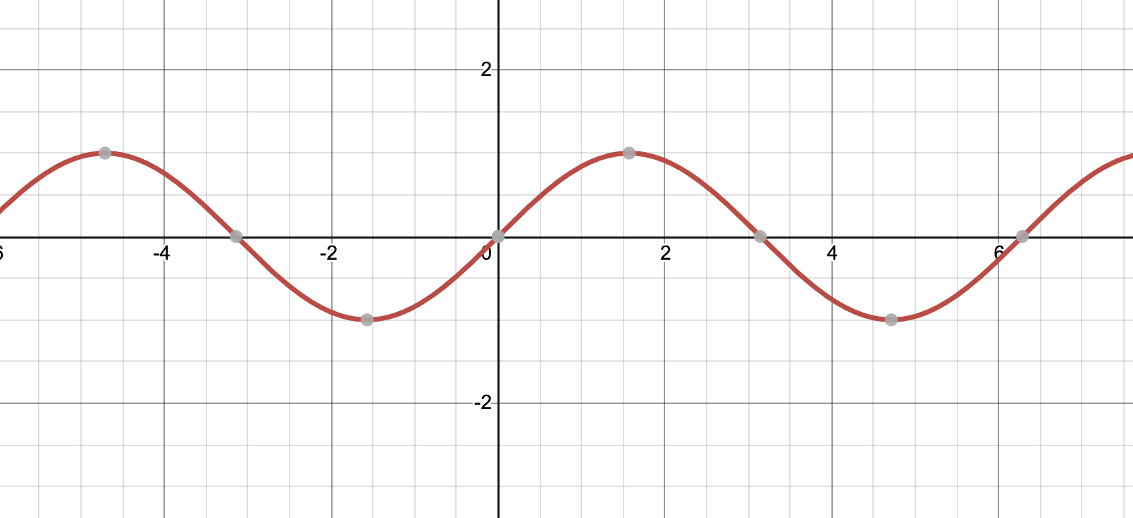
The sine function \(f(x)=sin(x)\) is not invertible in the domain \([\infty, -\infty]\). This is because values of \(x\) separated by \(\frac{\pi}{2}\) radians output the same value.
For the function \(f(x)=sin(x)\) to be invertible, we restrict its domain to \([-\frac{\pi}{2},\frac{\pi}{2}]\). You can easily see that in the range \([-\frac{\pi}{2},\frac{\pi}{2}]\), the sine function is monotonic (in this case, increasing).
This also leads us to an important practice: that of explicitly defining the region of the domain of the function where it is monotonic. In most cases, excluding the problematic areas of the domain, allows us to apply stricter conditions to a local area of a function, which would not be possible if the function was considered at a global scale.
Function Inverses in Higher Dimensions
What if we wish to extend this to the two-dimensional case? We now have a function \(F:\mathbb{R}^2 \rightarrow \mathbb{R}^2\). I said “a function”, but it is actually a vector of two functions. An elementary function returns a single scalar value, and to get two values (remember, \(\mathbb{R}^2\)) for our output vector, we need two functions. Let us write this as:
\[F(X)=\begin{bmatrix} f_1(x_1, x_2) \\ f_2(x_1, x_2) \end{bmatrix} \\ f_1(x_1, x_2)=x_1+x_2 \\ f_2(x_1, x_2)=x_1-x_2 \\ \Rightarrow F(X)= \begin{bmatrix} 1 && 1 \\ 1 && -1 \end{bmatrix}\]where \(X=(x_1,x_2)\). I have simply rewritten the functions in matrix form above. What is the inverse of this function? We can simply compute the inverse of this matrix to get the answer. I won’t show the steps here (I did this using augmented matrix Gaussian Elimination), but you can verify yourself that the inverse \(F^{-1}\) is:
\[F^{-1}(X)=\begin{bmatrix} \frac{1}{2} && \frac{1}{2} \\ \frac{1}{2} && -\frac{1}{2} \\ \end{bmatrix}\]This can be extended to all higher dimensions, obviously.
Let us repeat the same question as in the one-dimensional case: when is the function \(F\) not invertible? We need to make our definition a little more sophisticated in the case of multivariable functions; the new requirement is that all its partial derivatives always be invertible. Stated this way, this implies that the the gradient of the function (Jacobian) \(\nabla F\) be invertible over the entire region of interest.
Briefly, we’re looking at \(n\) equations with \(n\) unknowns, with all linearly independent column vectors. Linear independence is a necessary condition for invertibility.
We are now ready to state the Inverse Function Theorem (well, the important part).
Inverse Function Theorem
The Inverse Function Theorem states that:
In the neighbourhood of a domain around \(x_0\) of a function \(F\) which is known to be continuously differentiable, if the derivative of the function \(DF(x_0)\) is invertible, then there exists an inverse function \(F^{-1}\) which exists in that same neighbourhood such that \(F^{-1}(F(x_0))=x_0\).
The theorem also gives us information about what the derivative of the inverse function, but we’ll not delve into that aspect for the moment. Any textbook on Vector Calculus should have the relevant results.
This is a very informal definition of the Inverse Function Theorem, but it conveys the most important part, namely: if the derivative of a function is invertible in some neighbourhood of \(x_0\), there exists an inverse of the function itself in that neighbourhood.
The reason we stress a lot on the word neighbourhood is that a lot of functions are not necessarily continuously differentiable, especially for nonlinear functions. Linear functions look the same as their derivatives at every point, which is why we didn’t need to worry about taking the derivative of \(f(x)=2x\) in our initial example.
The Inverse Function Theorem obviously applies to linear functions, but its real value lies in applying to nonlinear functions, where the neighbourhood is taken to be infinitesmal, which then leads us to the definition of the manifold, which we have talked about in Vector Calculus: Lagrange Multipliers, Manifolds, and the Implicit Function Theorem.
Implicit Function Theorem
What can we say about systems of functions which have \(n\) unknowns, but less than \(n\) equations? The Implicit Function Theorem gives us an answer to this; think of it as a more general version of the Inverse Function Theorem.
Much of the mechanics implied by this theorem is covered in Vector Calculus: Lagrange Multipliers, Manifolds, and the Implicit Function Theorem. However, here we take a big-picture view.
Suppose we have \(m+n\) unknowns and \(n\) equations. Thus, we will have \(n\) pivotal variables, corresponding to \(n\) linearly independent column vectors of this system of linear equations. This means that \(n\) pivotal variables can be expressed in terms of \(m\) free variables. Let us call the \(m\) free variables \(U=(u_1, u_2,..., u_m)\), and the \(n\) pivotal variables \(V=(v_1, v_2, ..., v_n)\).
Let us consider the original function \(F_{old}\).
\[F_{old}(U,V)=\begin{bmatrix} f_1(u_1, u_2, u_3, ..., u_m, v_1, v_2, v_3, ..., v_n) \\ f_2(u_1, u_2, u_3, ..., u_m, v_1, v_2, v_3, ..., v_n) \\ f_3(u_1, u_2, u_3, ..., u_m, v_1, v_2, v_3, ..., v_n) \\ \vdots \\ f_n(u_1, u_2, u_3, ..., u_m, v_1, v_2, v_3, ..., v_n) \end{bmatrix}\]The new function \(F_{new}\) is what we obtain once we have expressed \(V\) in terms of only \(U\). It looks like this:
\[F_{new}(U)=\begin{bmatrix} u_1 \\ u_2 \\ u_3 \\ \vdots \\ u_m \\ \phi_1(u_1, u_2, u_3, ..., u_m) \\ \phi_2(u_1, u_2, u_3, ..., u_m) \\ \phi_3(u_1, u_2, u_3, ..., u_m) \\ \vdots \\ \phi_n(u_1, u_2, u_3, ..., u_m) \end{bmatrix}\]Note that the original formulation had a function F_{old} which transformed the full set \((U,V)\) into a new vector. The new formulation now has \(m\) free variables which stay unchanged after the transform, and \(n\) pivotal variables \(V\) which are mapped from \(U\) with a new set of functions \(\Phi=(\phi_1,\phi_2,...,\phi_n,)\).
Now, instead of asking: “Is there an inverse of the function \(F_{old}\)?”, we ask: “Is there an inverse of the function \(F_{new}\)?”
The situation is illustrated below.
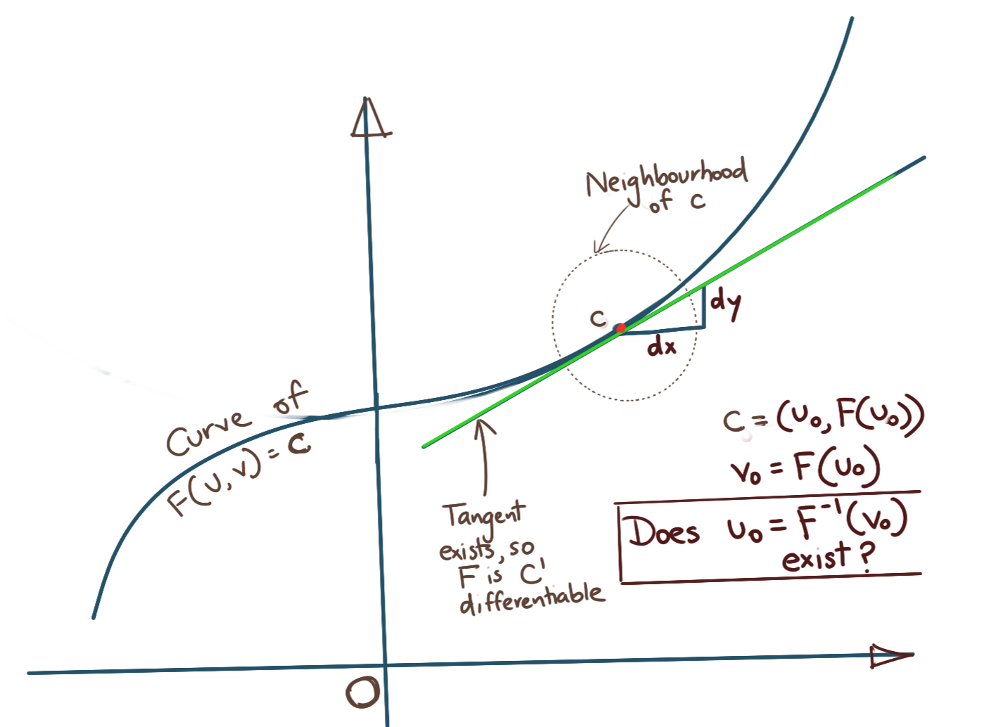
The Implicit Function Theorem states that if a mapping \(F_{old}(U,F_{new}(U))\) exists for a point \(c=(U_0, F_{new}(U_0))\) such that:
- \[\mathbf{F_{old}(c)=0}\]
- \(F_{old}(c)\) is first order differentiable (\(C^1\) differentiable)
- The derivative of \(F_{old}\) is invertible, implying \(L\) is also invertible, where \(L\) is defined as below:
then, the following holds true:
- There exists an inverse mapping \(F_{new}^{-1}\) for \(F_{new}\) such that \(F_{old}(F_{new}^{-1}(V), V)=0\) in the neighboourhood of \(c\)
- There is a neighbourhood of \(c\) where this linear relationship holds for \(F(c)=0\).
The above is the same statement as the one made by the Inverse Function Theorem, except that the system of linear equations in that scenario was completely determined. In the case of the Implicit Function Theorem, the system is underdetermined.
Note on the Derivative Matrix
Let us look at the matrix \(L\) defined above. Here, we have added padded the derivatives with the zero matrix and an identity matrix to make the whole matrix \(L\), square.
For simple linear surfaces, simply finding the inverse of the system of linear equations is enough, since as I noted, the gradient vector is the same as the surfce normal globally, but that is not true for “lumpy” functions globally. It is true for a neighbourhood \(x_0\). But what is the size of this neighbourhood such that the derivative approximates the actual function reasonably well?
Put another way, what is the size of the neighbourhood, where the first derivative does not change too fast for it to be useful in approximating the actual function? This requires the derivative satisfying the Lipschitz Condition, which is a way of putting a strong guarantee on continuous differentiability.
We will not go into the details of how this condition is satisfied, but only state that calculating a metric associated with this condition, requires us to compute \(L^{-1}\).
We know that \((D_1F_{old}, D_2F_{old}, D_3F_{old}, ..., D_nF_{old})\) is \(n \times n\) and is invertible, because we know that there are \(n\) linearly independent columns in \(F_{old}\).
The matrix \(L\) has the block form:
\[L= \begin{bmatrix} A && C \\ 0 && B \end{bmatrix}\]where \(A\) and \(B\) are invertible, but \(C\) need not be. To see why this results in \(L\) being invertible, see Intuitions around Matrix Multiplications.