Quadratic Optimisation: Lagrangian Dual, and the Karush-Kuhn-Tucker Conditions

Avishek Sen Gupta on 10 May 2021

---

This article concludes the (very abbreviated) theoretical background required to understand Quadratic Optimisation. Here, we extend the Lagrangian Multipliers approach, which in its current form, admits only equality constraints. We will extend it to allow constraints which can be expressed as inequalities.

Much of this discussion applies to the general class of Convex Optimisation; however, I will be constraining the form of the problem slightly to simplify discussion. We have already developed most of the basic mathematical results (see Quadratic Optimisation Concepts) in order to fully appreciate the implications of the Karush-Kuhn-Tucker Theorem.

Convex Optimisation solves problems framed using the following standard form:

Minimise (with respect to \(x\)), \(\mathbf{f(x)}\)

subject to:

\(\mathbf{g_i(x)\leq 0, i=1,...,n}\)
\(\mathbf{h_i(x)=0, i=1,...,m}\)

where:

• \(\mathbf{f(x)}\) is a convex function
• \(\mathbf{g_i(x)}\) are convex functions
• \(\mathbf{h_i(x)}\) are affine functions.

For Quadratic Optimisation, the extra constraint that is imposed is: \(g_i(x)\) is are also affine functions. Therefore, all of our constraints are essentially linear.

For this discussion, I’ll omit the equality constraints \(h_i(x)\) for clarity; any equality constraints can always be converted into inequality constraints, and become part of \(g_i(x)\).

Thus, this is the reframing of the Quadratic Optimisation problem for the purposes of this discussion.

Minimise (with respect to \(x\)), \(\mathbf{f(x)}\)

subject to: \(\mathbf{g_i(x)\leq 0, i=1,...,n}\)

where:

• \(\mathbf{f(x)}\) is a convex function
• \(\mathbf{g_i(x)}\) are affine functions

Karush-Kuhn-Tucker Stationarity Condition

We have already seen in Vector Calculus: Lagrange Multipliers, Manifolds, and the Implicit Function Theorem that the gradient vector of a function can be expressed as a linear combination of the gradient vectors of the constraint manifolds.

\[\mathbf{ Df=\lambda_1 Dh_1(U,V)+\lambda_2 Dh_2(U,V)+\lambda_3 Dh_3(U,V)+...+\lambda_n Dh_n(U,V) }\]

We can rewrite this as:

\[\mathbf{ Df(x)=\sum_{i=1}^n\lambda_i.Dg_i(x) } \\ \Rightarrow f(x)=\sum_{i=1}^n\lambda_i.g_i(x)\]

where \(x=(U,V)\). We will not consider the pivotal and non-pivotal variables separately in this discussion.

In this original formulation, we expressed the gradient vector as a linear combination of the gradient vector(s) of the constraint manifold(s). We can bring everything over to one side and flip the signs of the Lagrangian Multipliers to get the following:

\[Df(x)+\sum_{i=1}^n\lambda_i.Dg_i(x)=0\]

Since the derivatives in this case represent the gradient vectors, we can rewrite the above as:

\[\mathbf{ \begin{equation} \nabla f(x)+\sum_{i=1}^n\lambda_i.\nabla g_i(x)=0 \label{eq:kkt-1} \end{equation} }\]

This expresses the fact that the gradient vector of the tangent space must be opposite (and obviously parallel) to the direction of the gradient vector of the objective function. All it really amounts to is a change in the sign of the multipliers \(\lambda_i\); we do this so that the Lagrange multiplier terms act as penalties when the constraints \(g_i(x)\) are violated. We will see this in action when we explore the properties of the Lagrangian in the next few sections.

The identity \(\eqref{eq:kkt-1}\) is the Stationarity Condition, one of the Karush-Kuhn-Tucker Conditions.

Active and Inactive Constraints

In Quadratic Optimisation, \(g_i(x)|i=1,2,...,n\) represent the constraint functions. An important concept to get an intuition about, is the difference between dealing with pure equality constraints and inequality cnstraints.

The diagram below shows an example where all the constraints are equality constraints.

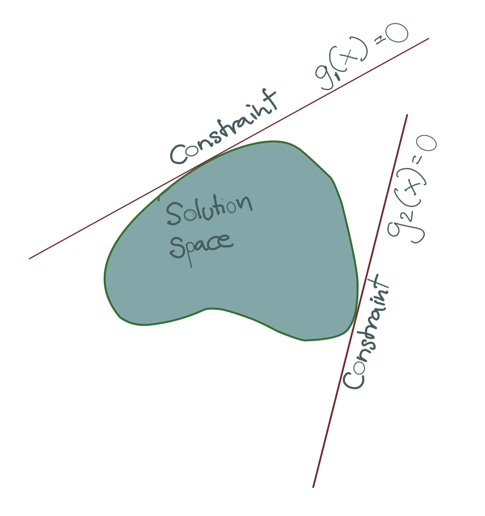
There are two points to note.

• All equality constraints are expressed in the form \(g_i(x)=0\) and they all must be satisfied simultaneously.
• All equality constraints, being affine, must be tangent to the objective function surface, since only then can the gradient vector of the solution be expressed as the Lagrangian combination of these tangent spaces.

The situation changes when inequality constraints are involved. Here is another rough diagram to demonstrate. The y-coordinate represents the image of the objective function \(f(x)\). The x-coordinate represents the image of the constraint function \(g(x)\), i.e., the different values \(g(x)\) can take for different values of \(x\).

The equality condition in this case maps to the y-axis, since that corresponds to \(g(x)=0\). However, we’re dealing with inequality constraints here, namely, \(g(x) \leq 0\); thus the viable space of solutions for \(f(x)\) are all to the left of the y-axis.

As you can see, since \(g(x)\leq 0\), the solution is not required to touch the level set of the constraint manifold corresponding to zero. Such solutions might not be the optimal solutions (we will see why in a moment), but they are viable solutions nevertheless.

We now draw two example solution spaces with two different shapes.

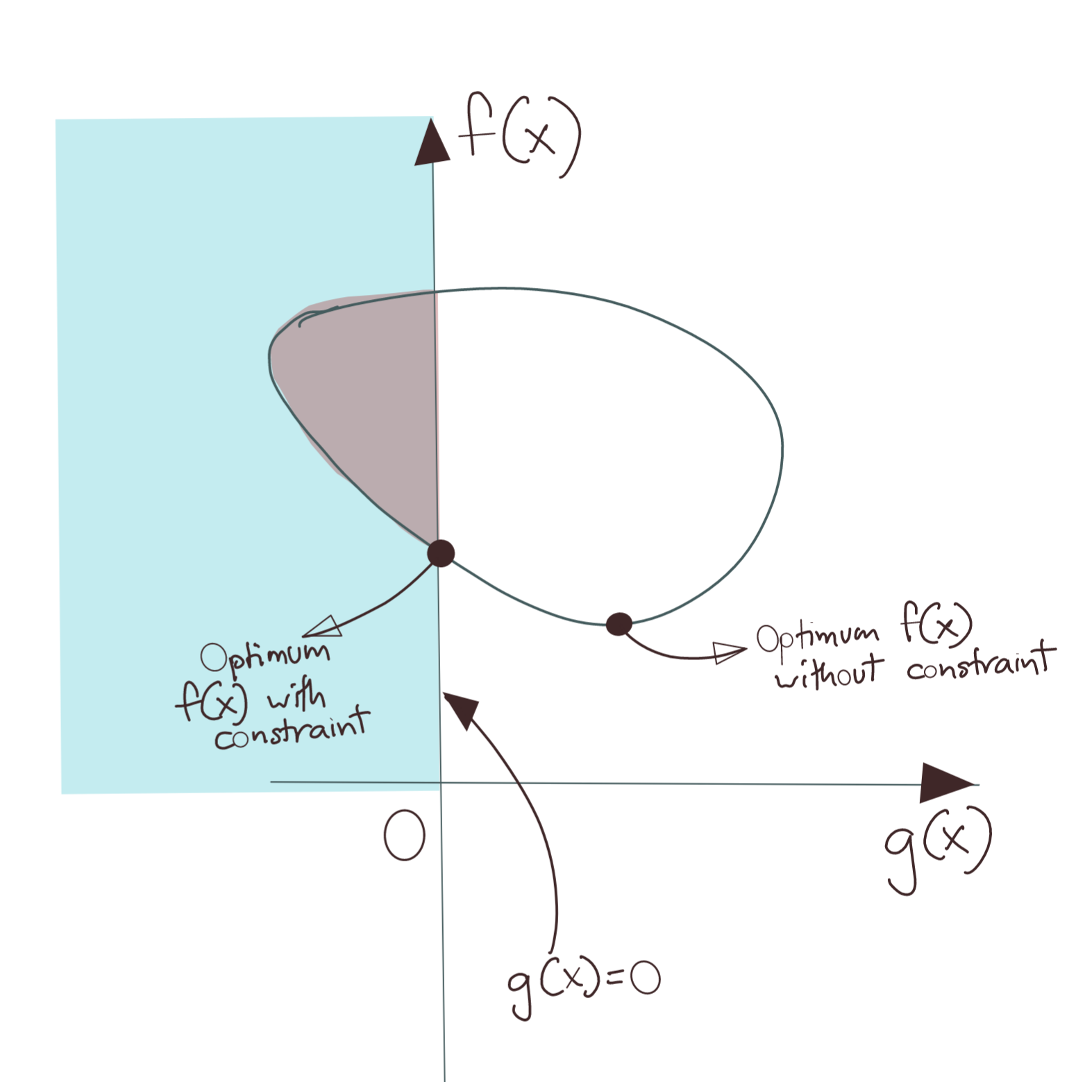
In the first figure, the global minimum of \(f(x)\) violates the constraint since it lies in the \(g(x)>0\). Thus, we cannot pick that; we must pick minimum \(f(x)\) that does not violate the constraint \(g(x)\leq 0\). This point in the diagram lies on the y-axis, i.e., on \(g(x)=0\). The constraint \(g(x)\leq 0\) in this scenario is considered an active constraint.

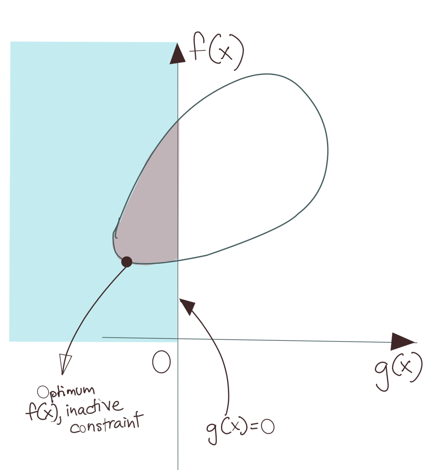
Contrast this with the diagram above. Here, the shape of the solution space is different. The minimum \(f(x)\) lies within the \(g(x)\leq 0\) zone. This means that even if we minimise \(f(x)\) without regard to the constraint \(g(x)\leq 0\), we’ll still get the minimum solution which still satisfies the constraint. In this scenario, we call \(g(x)\leq 0\) an inactive constraint. This implies that in this scenario, we do not even need to consider the constraint \(g_i(x)\) as part of the objective function. As you will see, after we define the Lagrangian, this can be done by setting the corresponding Lagrangian multiplier to zero.

The Lagrangian

We now have the machinery to explore the Lagrangian Dual in some detail. We will first consider the Lagrangian of a function. The Lagrangian form is simply restating the Lagrange Multiplier form as a function \(L(X,\lambda)\), like so:

\[L(x,\lambda)=f(x)+\sum_{i=1}^n\lambda_i.g_i(x)\text{ such that }\lambda_i\geq 0 \text{ and } g_i(x)\leq 0\]

Let us note these conditions from the above identity:

\[\begin{equation} \mathbf{ g_i(x)\leq 0 \label{eq:kkt-4} } \end{equation}\] \[\begin{equation} \mathbf{ \lambda_i\geq 0 \label{eq:kkt-3} } \end{equation}\]

• Primal Feasibility Condition: The inequality \(\eqref{eq:kkt-4}\) is the Primal Feasibility Condition, one of the Karush-Kuhn-Tucker Conditions.
• Dual Feasibility Condition: The inequality \(\eqref{eq:kkt-3}\) is the Dual Feasibility Condition, one of the Karush-Kuhn-Tucker Conditions.

We have simply moved all the terms of the Lagrangian formulation onto one side and denoted it by \(L(x,\lambda)\), like we talked about when concluding the Stationarity Condition.

Note that differentiating with respect to \(x\) and setting it to zero, will get us back to the usual Vector Calculus-motivated definition, i.e.:

\[D_xL= \mathbf{ \nabla f-{[\nabla G]}^T\lambda }\]

where \(G\) represents \(n\) constraint functions, \(\lambda\) represents the \(n\) Lagrange multipliers, and \(f\) is the objective function.

The Primal Optimisation Problem

We will now explore the properties of the Lagrangian, both analytically, as well as geometrically.

Remembering the definition of the supremum of a function, we find the supremum of the Lagrangian with respect to \(\lambda\) (that is, to find the supremum in each case, we vary the value of \(\lambda\)) to be the following:

\[sup_\lambda L(x,\lambda)=\begin{cases} f(x) & \text{if } g_i(x)\leq 0 \\ \infty & \text{if } g_i(x)>0 \end{cases}\]

Remember that \(\mathbf{\lambda \geq 0}\).

Thus, for the first case, if \(g_i(x) \leq 0\), the best we can do is set \(\lambda=0\), since any other non-negative value will not be the supremum.

In the second case, if \(g(x)>0\), the supremum of the function can be as high as we like as long as we keep increasing the value of \(\lambda\). Thus, we can simply set it to \(\infty\), and the corresponding supremum becomes \(\infty\).

We can see that the function \(sup_\lambda L(x)\) incorporates the constraints \(g_i(x)\) directly, there is a penalty of \(\infty\) for any constraint which is violated. Therefore, the original problem of minimising \(f(x)\) can be equivalently stated as:

\[\text{Minimise (w.r.t. x) }sup_\lambda L(x,\lambda) \\ \text{where } L(x,\lambda)=f(x)+\sum_{i=1}^n\lambda_i.g_i(x)\]

Equivalently, we say:

\[\text{Find }\mathbf{inf_x\text{ }sup_\lambda L(x,\lambda)} \\ \text{where } L(x,\lambda)=f(x)+\sum_{i=1}^n\lambda_i.g_i(x)\]

This is referred to in the mathematical optimisation field as the primal optimisation problem.

Karush-Kuhn-Tucker Complementary Slackness Condition

We previously discussed the two possible scenarios when optimising with constraints: either a constraint is active, or it is inactive.

• Constraint is active: This implies that the optimal point \(x^*\) lies on the constraint manifold. Thus, \(\mathbf{g_i(x^*)=0}\). Correspondingly, \(\mathbf{\lambda_i g(x^*)=0}\).
• Constraint is inactive: This implies that the optimal point \(x^*\) does not lie on the constraint manifold, but somewhere inside. Thus, \(\mathbf{g_i(x^*)<0}\). However, this also means that we can optimise \(f(x)\) without regard to the constraint \(g_i(x)\). The best way to get rid of this constraint then, is to set the corresponding Lagrange multiplier \(\mathbf{\lambda_i=0}\). Correspondingly, \(\mathbf{\lambda_i g(x^*)=0}\) again (albeit for different reasons from the active constraint case).

Thus, we may conclude that all \(\lambda_i g_i(x)\) terms in the Lagrangian must be zero, regardless of whether the corresponding constraint is active or inactive.

Mathematically, this implies:

\[\begin{equation} \mathbf{ \sum_{i=1}^n\lambda_i.g_i(x)=0 \label{eq:kkt-2} } \end{equation}\]

The identity \(\eqref{eq:kkt-2}\) is termed the Complementary Slackness Condition, one of the Karush-Kuhn-Tucker Conditions.

The Karush-Kuhn-Tucker Conditions

We are now in a position to summarise all the Karush-Kuhn-Tucker Conditions. The theorem states that for the optimisation problem given by:

\[\mathbf{\text{Minimise}_x \hspace{3mm} f(x)}\]

if the following conditions are met for some \(x^*\):

1. Primal Feasibility Condition

\(\mathbf{g_i(x^*)\leq 0}\)

2. Dual Feasibility Condition

\(\mathbf{\lambda_i\geq 0}\)

3. Stationarity Condition

\(\mathbf{\nabla f(x^*)+\sum_{i=1}^n\lambda_i.\nabla g_i(x^*)=0}\)

4. Complementary Slackness Condition

\(\mathbf{\sum_{i=1}^n\lambda_i.g_i(x^*)=0}\)

then \(x^*\) is a local optimum.

The Dual Optimisation Problem

We already know from the Max-Min Inequality that:

\[\mathbf{\sup_y \text{ inf}_x f(x,y)\leq \inf_x \text{ sup}_y f(x,y)} \text{ }\forall x,y\in\mathbb{R}\]

Since this is a general statement about any \(f(x,y)\), we can apply this inequality to the Primal Optimisation Problem, i.e.:

\[\sup_\lambda \text{ inf}_x L(x,\lambda) \leq \inf_x \text{ sup}_\lambda L(x,\lambda)\]

The right side is the Primal Optimisation Problem, and the left side is known as the Dual Optimisation Problem, and in this case, the Lagrangian Dual.

To understand the fuss about the Lagrangian Dual, we will begin with the more restrictive case where equality holds for the Max-Min Inequality, and later discuss the more general case and its implications. For this first part, we will assume that:

\[\sup_\lambda \text{ inf}_x L(x,\lambda) = \inf_x \text{ sup}_\lambda L(x,\lambda)\]

Let’s look at a motivating example. This is the graph of the Lagrangian for the following problem:

\[\text{Minimise}_x f(x)=x^2 \\ \text{subject to: } x \leq 0\]

The Lagrangian in this case is given by:

\[L(x,\lambda)=x^2+\lambda x\]

This is the corresponding graph of \(L(x,\lambda)\).

Let us summarise a few properties of this graph.

• The function is convex in \(x\): Assume \(\lambda=C\) is a constant, then the function has the form \(\mathbf{x^2+Cx}\) which is a family of parabolas. A parabola is a convex function, thus the result follows.
• The function is concave in \(\lambda\): Assume that \(x=C\) and \(x^2=K\) are constants, then the function has the form \(\mathbf{C\lambda+K}\), which is the general form of affine functions. Affine functions are both convex and concave, but we will be drawing more conclusions based on their concave nature, so we will simply say that the Lagrangian is concave in \(\lambda\). Thus, the Lagrangian is also a family of concave functions.
• As a direct consequence of the Lagrangian being a family of concave functions, we can say that the pointwise infimum of the Lagrangian is a concave function. We established this result in Quadratic Optimisation Concepts. This result is irrespective of the shape of the Lagrangian in the direction of \(x\).

This is important because it allows us to frame the Lagrangian of a Quadratic Optimisation as a concave-convex function. This triggers a whole list of simplifications, some of which I list below (we’ll discuss most of them in succeeding sections).

• Guarantee of a saddle point
• Zero duality gap by default
• No extra conditions for Strong Duality

Geometric Intuition of the Lagrange Dual Problem

Let us look at the geometric interpretation of the Lagrangian Dual. For this discussion, we will assume that the constraints are active. The Lagrangian itself is:

\[L(x,\lambda)=f(x)+\sum_{i=1}^n\lambda_i.g_i(x)\text{ such that }\lambda_i\geq 0 \text{ and } g_i(x)\leq 0\]

For the purposes of the discussion, let’s assume one constraint, so that the Lagrangian is now:

\[L(x,\lambda)=f(x)+\lambda.g(x)\text{ such that }\lambda\geq 0 \text{ and } g(x)\leq 0\]

Let us map \(f(x)\) (y-coordinate) and \(g(x)\) (x-coordinate), treating them as variables themselves. Then we see that the Lagrangian is of the form:

\[C=\lambda.g(x)+f(x) \\ \Rightarrow f(x)=-\lambda.g(x)+C\]

This is the equation of a straight line, with slope \(-\lambda\) and y-intercept \(C\). Note that \(C\) in this case represents the Lagrangian objective function.

Let’s walk through the Lagrangian maximisation-minimisation procedure step-by-step. The procedure is:

\[\sup_\lambda \text{ inf}_x L(x,\lambda)\]

There are two important points to note here:

• We have restricted \(\lambda\geq 0\). Therefore the slope of the Lagrangian is always negative.
• Moving this line to the left decreases its y-intercept, in this case, \(C\).

1. Infimum with respect to \(x\)

The first step is \(\text{ inf}_x L(x,\lambda)\), which translates to:

\[\text{ inf}_x \lambda.g(x)+f(x)\]

• For a given value of \(\lambda\), find the lowest possible \(C\), such that all the constraints are still respected.

Geometrically, this means taking the line \(f(x)=\lambda g(x)\), and moving it as far to the left as possible while it has at least one point in \(G\).

Algebraically, this gives us:

\[0=\lambda.\frac{dg(x)}{dx}+\frac{df(x)}{dx} \\ \Rightarrow \frac{df(x)}{dx}=-\lambda.\frac{dg(x)}{dx} \\ \Rightarrow \nabla f(x)=-\lambda.\nabla g(x)\]

This gives us the condition for such a minimisation to be possible, which, as you must have guessed, simply restates the Kuhn-Tucker Stationarity Condition.

The situation looks like below.

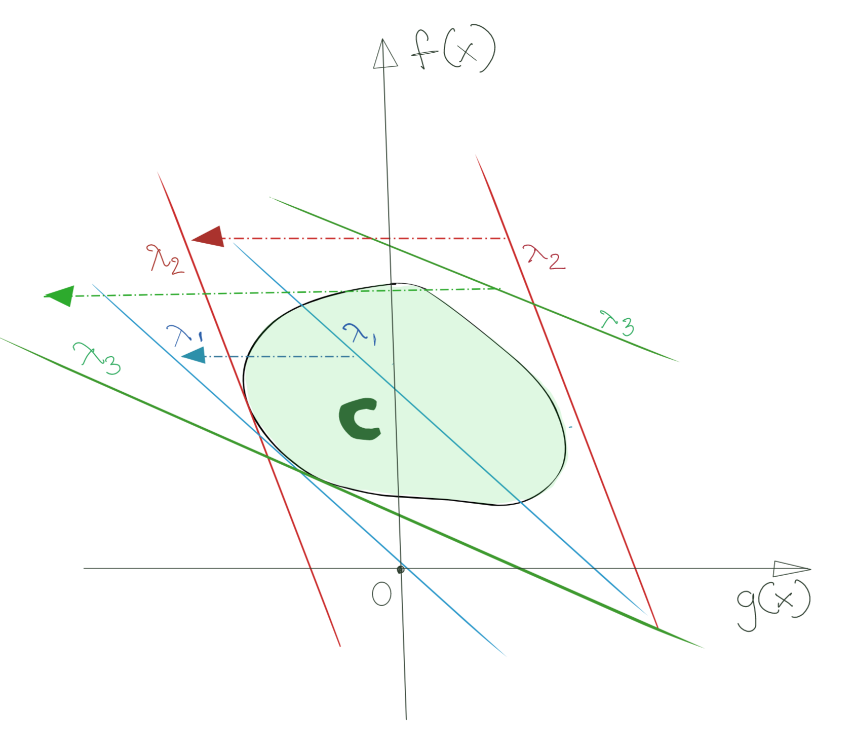
The important thing to note is that as a result of taking the infimum, all the Lagrangians are now supporting hyperplanes of \(G\).

Also, because \(\lambda\geq 0\) and also due to how the infimum works, none of the supporting hyperplanes touch \(G\) in the first quadrant (positive); they have all moved as far left as possible, and are effectively tangent to \(G\) at \(g(x)\leq 0\).

As you see below, this operation holds true even for nonconvex sets.

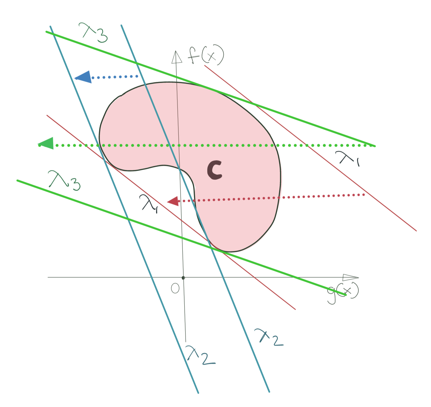
The infimum operation tells us what the supporting hyperplane for the convex set looks like for a given value of \(\lambda\). Obviously, this also implies that the Lagrangian is tangent to \(G\). This is expressed by the fact that the gradient vector of \(f(x)\) is parallel and opposite to the gradient vector of the constraint \(g(x)\).

Take special note of the Lagrangian line for \(\lambda_1\) in the nonconvex set scenario; we shall have occasion to revisit it very soon.

1. Supremum with respect to \(\lambda\)

The above infimum (minimisation) operation has given us the Lagrangian in terms of \(\lambda\) only. This family of Lagrangians is represented by \(\text{ inf}_x \lambda.g(x)+f(x)\).

Geometrically, you can assume that you have an infinite set of Lagrangians, one for every value of \(\lambda\), each of them a supporting hyperplane for the \([g(x), f(x)]\) set.

Now, to actually find the optimum point, we’d like to select the supporting hyperplane that has the maximum corresponding cost \(C\), or y-intercept. Algebraically, this implies finding \(\text{ inf}_\lambda \text{ inf}_x \lambda.g(x)+f(x)\).

Note that the Lagrangian is concave in \(\lambda\), thus the minimisation has also given us a concave problem to solve. In this case, we will be maximising this concave problem (which corresponds to minimising a convex problem).

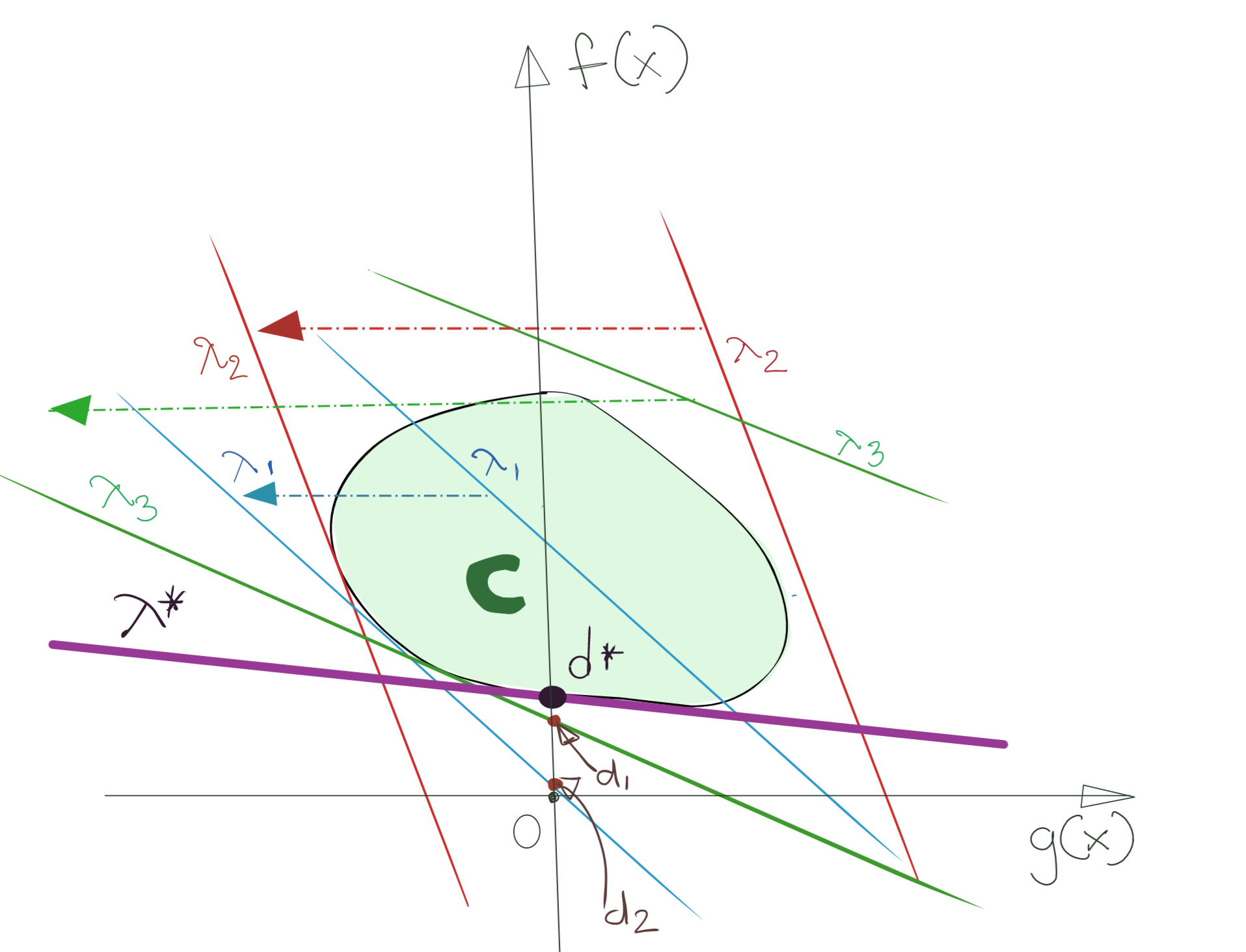
In the diagram above, I’ve marked the winning supporting hyperplane, thicker. For this hyperplane with its value of \(\lambda^*\), the y-intercept (the Lagrangian cost) is maximised. This critical point is marked \(d^*\).

Strong Duality

The interesting (and useful) thing to note is that if you were to solve the Primal Optimisation Problem instead of the Lagrangian Dual Problem, or even the original optimisation problem in the standard Quadratic Programming form, you will get the same result as \(d^*\).

This is the result of the function being concave in \(\lambda\) and convex in \(x\), implying the existence of a saddle point. This is also the situation where the equality clause of the Max-Min Inequality holds.

Weak Duality and the Duality Gap

I’d purposefully omitted the result of finding the supremum for the nonconvex case in the previous section. This is because the nonconvex scenario is what shows us the real difference between the Primal Optimisation Problem and its Lagrangian Dual.

The winning supporting hyperplane for the nonconvex set is shown below.

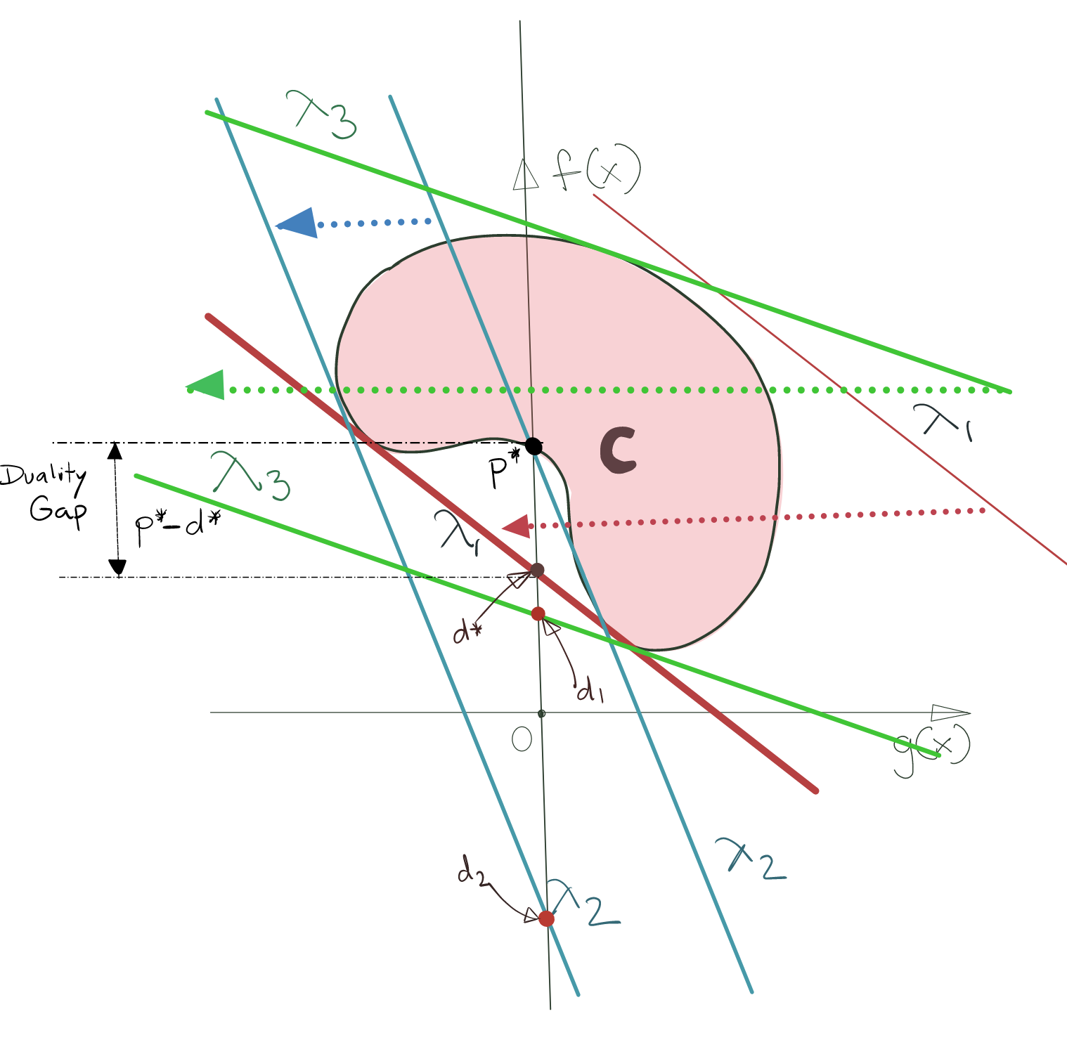
The solution for the Lagrangian Dual Problem is marked \(d^*\), and the solution for the Primal Optimisation Problem is marked \(p^*\). As you can clearly see, \(d^*\) and \(p^*\) do not coincide.

The dual solution is in this case, is not the actual solution, but it provides a lower bound on \(p^*\), i.e., if we can compute \(d^*\), we can use it to decide if the solution by an optimisation algorithm is “good enough”. It is also a validation that we are not searching in an infeasible area of the solution space.

This is the situation where the inequality condition of the Max-Min Inequality holds.

The difference between the \(p^*\) and \(d^*\) is called the Duality Gap. Obviously, the duality gap is zero when conditions of Strong Duality are satisfied. When these conditions for Strong Duality are not satisfied, we say that Weak Duality holds.

Conditions for Strong Duality

There are many different conditions which, if satisfied by themselves, guarantee Strong Duality. In particular, textbooks cite Slater’s Constraint Qualification very frequently, and the Linear Independence Constraint Qualification also finds mention.

The above-mentioned constraint qualifications assume that the constraints are nonlinear.

However, for our current purposes, if we assume that the inequality constraints are affine functions, we do not need to satisfy any other condition: the duality gap will be zero by default under these conditions; the optimum dual solution will always equal the optimal primal solution, i.e., \(p^*=d^*\).

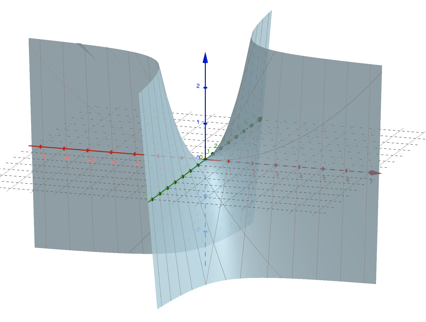
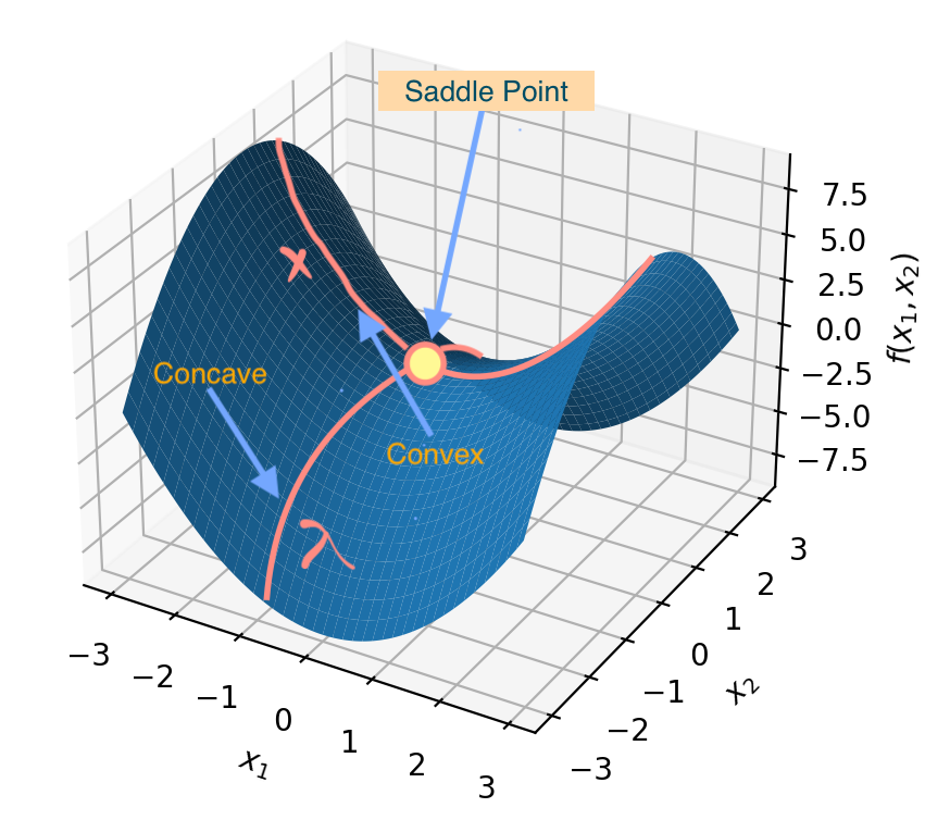
This also guarantees the existence of a saddle point in the solution of the Lagrangian. A saddle point of a function \(f(x,y)\) is defined as a point (x^,y^) which satisfies the following condition:

\[f(x^*,\bigcirc)\leq f(x^*,y^*)\leq f(\bigcirc, y^*)\]

where \(\bigcirc\) represents “any \(x\)” or “any \(y\)” depending upon its placement. Applying this to our objective function, we can write:

\[f(x^*,\bigcirc)\leq f(x^*,\lambda^*)\leq f(\bigcirc, \lambda^*)\]

The implication is that starting from the saddle point, the function slopes down in the direction of \(\lambda\), and slopes up in the direction of \(x\). The figure below shows the general shape of the Lagrangian with a convex objective function and affine (inequality and equality) constraints.

The reason this leads to Strong Duality is this: minimising \(f(x,\lambda)\) with respect to \(x\) first, then maximising with respect to \(\lambda\), takes us to the same point \((x^*,y^*)\) that would be reached, if we first maximise \(f(x,\lambda)\) with respect to \(\lambda\), then minimise with respect to \(\lambda\).

Mathematically, this implies that:

\[\mathbf{\sup_\lambda \text{ inf}_x f(x,\lambda)= \inf_x \text{ sup}_\lambda f(x,\lambda)}\]

thus implying that the Duality Gap is zero.

Notes

• Karush-Kuhn-Tucker Conditions use Farkas’ Lemma for proof.
• The Saddle Point Theorem is not proven here.

---