Gaussian Processes: Theory

Avishek Sen Gupta on 10 September 2021

---

In this article, we will build up our mathematical understanding of Gaussian Processes. We will understand the conditioning operation a bit more, since that is the backbone of inferring the posterior distribution. We will also look at how the covariance matrix evolves as training points are added.

Continuing from the roadmap set out in Road to Gaussian Processes and the intuition we built up in the first pass on Gaussian Processes in Gaussian Processes: Intuition, the requisite material you should be familiar with, is presented in the following articles.

• Geometry of the Multivariate Gaussian Distribution
• Gaussian Processes: Intuition

The following material will be covered:

• Conditioning a Bivariate Gaussian Distribution: Brute Force Derivation
• Schur Complements and Diagonalisation of Partitioned Matrices
• Factorisation of the Joint Gaussian Probability Distribution
• Evolution of the Covariance Matrix

Bivariate Gaussian Distribution: Brute Force Derivation

Before moving to the generalised method of proof, I feel it instructive to look at the Bivariate Gaussian Distribution. Apart from the fact that the results for the mean and covariance apply to the more general case, it is helpful to see the mechanics of the exercise starting with the eigendecomposed form of the covariance matrix, before introducing Schur Complements for the more general case.

To that end, we define the Bivariate Gaussian Distribution as:

\[\begin{equation} P(x,y)=K_0\cdot \exp\left( -\frac{1}{2} {(X-\mu)}^T\Sigma^{-1}(X-\mu)\right) \label{eq:bivariate-joint-gaussian} \end{equation}\]

where \(X\), \(\mu\), and \(\Sigma\) are defined as follows:

\[X = \begin{bmatrix} x \\ y \end{bmatrix} \\ \mu = \begin{bmatrix} \mu_x \\ \mu_y \end{bmatrix} \\\] \[\begin{equation} \Sigma = \begin{bmatrix} \Sigma_{11} && \Sigma_{12} \\ \Sigma_{21} && \Sigma_{22} \\ \end{bmatrix} \label{eq:covariance-matrix} \end{equation}\]

Note that \(\Sigma\) is necessarily symmetric. Furthermore, the covariance matrix can be decomposed into orthonormal eigenvectors like so:

\[\begin{equation} \Sigma= \begin{bmatrix} a && -b \\ b && a \\ \end{bmatrix} \cdot \begin{bmatrix} \lambda_1 && 0 \\ 0 && \lambda_2 \\ \end{bmatrix} \cdot \begin{bmatrix} a && b \\ -b && a \\ \end{bmatrix} \label{eq:covariance-eigendecomposition} \end{equation}\]

where \(\sqrt{a^2+b^2}=1\).

Then, multiplying out the expression in \(\eqref{eq:covariance-eigendecomposition}\) and equating the result to the terms in \(\eqref{eq:covariance-matrix}\) gives us the following:

\[\Sigma= \begin{bmatrix} \Sigma_{11} && \Sigma_{12} \\ \Sigma_{21} && \Sigma_{22} \\ \end{bmatrix} = \begin{bmatrix} \lambda_1 a^2 + \lambda_2 b^2 && ab(\lambda_1-\lambda_2) \\ ab(\lambda_1-\lambda_2) && \lambda_1 b^2 + \lambda_2 a^2 \end{bmatrix} \\ \Sigma_{11}=\lambda_1 a^2 + \lambda_2 b^2 \\ \Sigma_{12}=\Sigma_{21}=ab(\lambda_1-\lambda_2) \\ \Sigma_{22}=\lambda_1 b^2 + \lambda_2 a^2\]

Consequently, we can also write \(\Sigma^{-1}\) as:

\[\begin{equation} \Sigma^{-1}= \begin{bmatrix} a && -b \\ b && a \\ \end{bmatrix} \cdot \begin{bmatrix} \frac{1}{\lambda_1} && 0 \\ 0 && \frac{1}{\lambda_2} \\ \end{bmatrix} \cdot \begin{bmatrix} a && b \\ -b && a \\ \end{bmatrix} \label{eq:inverse-covariance} \end{equation}\]

Let us condition on \(y\), i.e., we set \(y=y_0\), and derive the resulting one-dimensional probability distribution in \(x\). The conditioning will then look like:

\[\begin{equation} P(x|y=y_0)=\frac{P(x,y)}{P(y=y_0)} \label{eq:conditional-distribution} \end{equation}\]

We have already defined \(P(x,y)\) in \(\eqref{eq:bivariate-joint-gaussian}\). The other expression \(P(y=y_0)\) then looks like this:

\[\begin{equation} P(y=y_0)=K_1\cdot \exp\left(-\frac{1}{2}\cdot\frac{ {(y_0-\mu_y)}^2}{\Sigma_{22}}\right) \\ P(y=y_0)=K_1\cdot \exp\left(-\frac{1}{2}\cdot\frac{ {(y_0-\mu_y)}^2}{\lambda_1 b^2 + \lambda_2 a^2}\right) \label{eq:y-condition} \end{equation}\]

Putting \(\eqref{eq:y-condition}\) and \(\eqref{eq:bivariate-joint-gaussian}\) into \(\eqref{eq:conditional-distribution}\), we get:

\[\begin{equation} P(x|y=y_0)=\frac{K_0\cdot \exp\left( -\frac{1}{2} {(X-\mu)}^T\Sigma^{-1}(X-\mu)\right)}{K_1\cdot \exp\left(-\frac{1}{2}\cdot\frac{ {(y_0-\mu_y)}^2}{\lambda_1 b^2 + \lambda_2 a^2}\right)} \\ =\frac{K_0}{K_1}\cdot\exp\left[-\frac{1}{2}\left( \begin{bmatrix} x-\mu_x && y_0-\mu_y \end{bmatrix} \cdot \begin{bmatrix} a && -b \\ b && a \\ \end{bmatrix} \cdot \begin{bmatrix} \frac{1}{\lambda_1} && 0 \\ 0 && \frac{1}{\lambda_2} \\ \end{bmatrix} \cdot \begin{bmatrix} a && b \\ -b && a \\ \end{bmatrix} \cdot \begin{bmatrix} x-\mu_x \\ y_0-\mu_y \end{bmatrix} - \frac{ {(y_0-\mu_y)}^2}{\lambda_1 b^2 + \lambda_2 a^2} \right) \right] \\ =\frac{K_0}{K_1}\cdot\exp\left[-\frac{1}{2}\left( \underbrace{ \begin{bmatrix} x-\mu_x && y_0-\mu_y \end{bmatrix} \cdot \begin{bmatrix} \frac{a^2}{\lambda_1}+\frac{b^2}{\lambda_2} && ab(\frac{1}{\lambda_1}-\frac{1}{\lambda_2}) \\ ab(\frac{1}{\lambda_1}-\frac{1}{\lambda_2}) && \frac{b^2}{\lambda_1}+\frac{a^2}{\lambda_2} \\ \end{bmatrix} \cdot \begin{bmatrix} x-\mu_x \\ y_0-\mu_y \end{bmatrix} }_A - \frac{ {(y_0-\mu_y)}^2}{\lambda_1 b^2 + \lambda_2 a^2} \right) \right] \label{eq:conditional-distribution-derivation} \end{equation}\]

Let us simplify \(A\), where:

\[A = \begin{bmatrix} x-\mu_x && y_0-\mu_y \end{bmatrix} \cdot \begin{bmatrix} \frac{a^2}{\lambda_1}+\frac{b^2}{\lambda_2} && ab(\frac{1}{\lambda_1}-\frac{1}{\lambda_2}) \\ ab(\frac{1}{\lambda_1}-\frac{1}{\lambda_2}) && \frac{b^2}{\lambda_1}+\frac{a^2}{\lambda_2} \\ \end{bmatrix} \cdot \begin{bmatrix} x-\mu_x \\ y_0-\mu_y \end{bmatrix}\]

Multiplying everything out in \(A\), we get:

\[A = \frac{ {(x-\mu_x)}^2(\lambda_2 a^2 + \lambda_1 b^2) - 2(x-\mu_x)(y_0-\mu_y)ab(\lambda_1 - \lambda_2) + {(y_0-\mu_y)}^2 (\lambda_2 b^2 + \lambda_1 a^2)}{\lambda_1\lambda_2} \\ = \frac {\lambda_2 a^2 + \lambda_1 b^2}{\lambda_1\lambda_2}\left[ \underbrace{ {(x-\mu_x)}^2 - \frac{2(x-\mu_x)(y_0-\mu_y)ab(\lambda_1 - \lambda_2)}{\lambda_2 a^2 + \lambda_1 b^2} }_{\text{Complete the Square}} + \frac{ {(y_0-\mu_y)}^2 (\lambda_2 b^2 + \lambda_1 a^2)}{\lambda_2 a^2 + \lambda_1 b^2}\right]\]

Completing the square above as indicated gives us:

\[A = \frac {\lambda_2 a^2 + \lambda_1 b^2}{\lambda_1\lambda_2} \left[{\left(x-\mu_x-\frac{(y_0-\mu_y)ab(\lambda_1-\lambda_2)}{\lambda_2 a^2 + \lambda_1 b^2}\right)}^2 - \frac { {(y_0-\mu_y)}^2 a^2 b^2 {(\lambda_1-\lambda_2)}^2 }{ {(\lambda_2 a^2 + \lambda_1 b^2)}^2} + \frac{ {(y_0-\mu_y)}^2 (\lambda_2 b^2 + \lambda_1 a^2)}{\lambda_2 a^2 + \lambda_1 b^2}\right] \\ = \frac {\lambda_2 a^2 + \lambda_1 b^2}{\lambda_1\lambda_2} \left[{\left(x-\mu_x-\frac{(y_0-\mu_y)ab(\lambda_1-\lambda_2)}{\lambda_2 a^2 + \lambda_1 b^2}\right)}^2 + \frac { {(y_0-\mu_y)}^2 {(a^2+b^2)}^2 \lambda_1 \lambda_2 }{ {(\lambda_2 a^2 + \lambda_1 b^2)}^2} \right]\]

However, remember that the \(\sqrt{a^2+b^2}=1\), thus we get:

\[A= \frac {\lambda_2 a^2 + \lambda_1 b^2}{\lambda_1\lambda_2} \left[{\left(x-\mu_x-\frac{(y_0-\mu_y)ab(\lambda_1-\lambda_2)}{\lambda_2 a^2 + \lambda_1 b^2}\right)}^2 + \frac { {(y_0-\mu_y)}^2 \lambda_1 \lambda_2 }{ {(\lambda_2 a^2 + \lambda_1 b^2)}^2} \right] \\ = \frac {\lambda_2 a^2 + \lambda_1 b^2}{\lambda_1\lambda_2} {\left(x-\mu_x-\frac{(y_0-\mu_y)ab(\lambda_1-\lambda_2)}{\lambda_2 a^2 + \lambda_1 b^2}\right)}^2 + \frac { {(y_0-\mu_y)}^2}{ \lambda_2 a^2 + \lambda_1 b^2}\]

Substituting the value of \(A\) back into \(\eqref{eq:conditional-distribution-derivation}\), we get:

\[\require{cancel} P(x|y=y_0)=\frac{K_0}{K_1}\cdot \exp\left( -\frac{1}{2} \frac {\lambda_2 a^2 + \lambda_1 b^2}{\lambda_1\lambda_2} {\left(x-\mu_x-\frac{(y_0-\mu_y)ab(\lambda_1-\lambda_2)}{\lambda_2 a^2 + \lambda_1 b^2}\right)}^2\right)\cdot\exp\left(\cancel{\frac { {(y_0-\mu_y)}^2}{ \lambda_2 a^2 + \lambda_1 b^2}} - \cancel{\frac { {(y_0-\mu_y)}^2}{ \lambda_2 a^2 + \lambda_1 b^2}}\right) \\ =\frac{K_0}{K_1}\cdot \exp\left( -\frac{1}{2} \frac {\lambda_2 a^2 + \lambda_1 b^2}{\lambda_1\lambda_2} {\left(x-\mu_x-\frac{(y_0-\mu_y)ab(\lambda_1-\lambda_2)}{\lambda_2 a^2 + \lambda_1 b^2}\right)}^2\right) \\ =\frac{K_0}{K_1}\cdot \exp\left( -\frac{1}{2} \frac {\lambda_2 a^2 + \lambda_1 b^2}{\lambda_1\lambda_2} {\left(x-\mu_x-\frac{(y_0-\mu_y)\Sigma_{12}}{\Sigma_{22}}\right)}^2\right) \\ P(x|y=y_0)=\frac{K_0}{K_1}\cdot \exp\left( -\frac{1}{2} {\left(\frac {\lambda_1\lambda_2}{\lambda_2 a^2 + \lambda_1 b^2}\right)}^{-1} {\left(x-\left[\mu_x+\frac{(y_0-\mu_y)\Sigma_{12}}{\Sigma_{22}}\right]\right)}^2\right)\]

The final expression gives us a one-dimensional Gaussian with mean and covariance as:

\[\begin{equation} \mu_{x|y=y_0}=\mu_x+\frac{(y_0-\mu_y)\Sigma_{12}}{\Sigma_{22}} \label{eq:bivariate-gaussian-mean} \end{equation}\] \[\begin{equation} \Sigma_{x|y=y_0}=\frac {\lambda_1\lambda_2}{\lambda_2 a^2 + \lambda_1 b^2} \label{eq:bivariate-gaussian-covariance} \end{equation}\]

More generally, as we will see in Factoring the Joint Probability Distribution(and you can verify yourself, especially the covariance expression), the mean and variance of the conditional probability are:

\[\begin{equation} \mu_{x|y=y_0}=\mu_x+(y_0-\mu_y){\Sigma_{22}}^{-1}\Sigma_{12} \label{eq:multivariate-gaussian-mean} \end{equation}\] \[\begin{equation} \Sigma_{x|y=y_0}=\Sigma_{11}-\Sigma_{12}{\Sigma_{22}}^{-1}\Sigma_{21} \label{eq:multivariate-gaussian-covariance} \end{equation}\]

You can verify that evaluation the expression \(\eqref{eq:multivariate-gaussian-covariance}\) indeed yields the expression for the conditioned covariance matrix of the Bivariate Gaussian in \(\eqref{eq:bivariate-gaussian-covariance}\).

As you will have also noticed, the derivation quickly becomes very complicated, and a general approach is needed to scale the proof to higher dimensions. This is the focus of the next topic.

Joint Distribution: Organising the Covariance Matrix

In the examples that we’ve used to generate the diagrams to build up our intuition so far, all the input points are assumed to be in \(\mathbb{R}\). Thus, there is a natural ordering of the input points, which is also reflected in their indexing in the covariance matrix. The variables in the covariance matrix (which represent individual input vectors) therefore use the matrix indices as their values. This is not going to be the case for vectors in \(\mathbb{R}^2\) and above, because there is no natural ordering that would exist between vectors in higher dimensions. In fact, even for \(\mathbb{R}\), the points need not exist in the matrix in the natural order that they would appear on the number line; all that would be needed then is to have some bookkeeping which maps the matrix indices to the correct vector value on the real number line. This mapping would then be used to do the actual plotting or presentation.

This will be particularly important to keep in mind, when we get into the proofs because we will be shuffling the order of the variables around, depending upon the variables we will be conditioning on.

We will now discuss the motivation for partitioning the covariance matrix. Let us assume we have \(N\) random variables \(X=\{x_1, x_2, ..., x_N\}\). The joint probability distribution of these random variables is then given by the covariance matrix as below:

\[P(x_1, x_2, \cdots, x_N)=K\cdot\exp\left(-\frac{1}{2}{(X-\mu_0)}^T\Sigma^{-1}(X-\mu_0)\right)\]

where the covariance matrix \(\Sigma\) is defined as below:

\[\Sigma= \begin{bmatrix} \kappa(x_1, x_1) && \kappa(x_1, x_2) && \cdots && \kappa(x_1, x_N) \\ \kappa(x_2, x_1) && \kappa(x_2, x_2) && \cdots && \kappa(x_2, x_N) \\ \kappa(x_3, x_1) && \kappa(x_3, x_2) && \cdots && \kappa(x_3, x_N) \\ \vdots && \vdots && \ddots && \vdots \\ \kappa(x_N, x_1) && \kappa(x_N, x_2) && \cdots && \kappa(x_N, x_N) \\ \end{bmatrix}\]

The similarity measure \(\kappa(x,y)\) is essentially a kernel function.

Now, let us pick an arbitrary set of random variables to fix (i.e., condition on). To be more concrete, the set of variables to condition on is \(X_T={x_{T1}, x_{T2}, x_{T3}, ..., x_{Tm}}\) (the \(T\) subscript stands for “Training”, since these are usually training data). The remaining variables that we do not condition are \(X_U={x_{U1}, x_{U2}, x_{U3}, ..., x_{Un}}\) (the \(U\) subscript stands for “Unconditioned”, these points usually end up being test data/real world data).

• It should be obvious that \(m+n=N\).
• The indices \(T1, T2, ...\) are not sequential. Neither are \(U1, U2, ...\)

Now we reorganise the original covariance matrix \(\Sigma\) by grouping the variables in \(X_U\) into one submatrix, and the ones in \(X_T\) into another submatrix. These submatrices form the diagonals of this new block diagonal matrix. Note that functionally, this reorganisation does not affect the properties of \(\Sigma\); it is still the original covariance matrix; it is just that the indices map to different random variables.

\[\begin{equation} \Sigma= \left[ \begin{array}{cccc|cccc} \kappa(x_{U1}, x_{U1}) & \kappa(x_{U1}, x_{U2}) & \cdots & \kappa(x_{U1}, x_{Un}) & \kappa(x_{U1}, x_{T1}) & \kappa(x_{U1}, x_{T2}) & \cdots & \kappa(x_{Un}, x_{Tm}) \\ \kappa(x_{U2}, x_{U1}) & \kappa(x_{U2}, x_{U2}) & \cdots & \kappa(x_{U2}, x_{Un}) & \kappa(x_{U2}, x_{T1}) & \kappa(x_{U2}, x_{T2}) & \cdots & \kappa(x_{Un}, x_{Tm}) \\ \vdots & \vdots & \ddots & \vdots & \vdots & \vdots & \ddots & \vdots \\ \kappa(x_{Un}, x_{U1}) & \kappa(x_{Un}, x_{U2}) & \cdots & \kappa(x_{Un}, x_{Un}) & \kappa(x_{Un}, x_{T1}) & \kappa(x_{Un}, x_{T2}) & \cdots & \kappa(x_{Un}, x_{Tm}) \\ \hline \kappa(x_{T1}, x_{U1}) & \kappa(x_{T1}, x_{U2}) & \cdots & \kappa(x_{T1}, x_{Un}) & \kappa(x_{T1}, x_{T1}) & \kappa(x_{T1}, x_{T2}) & \cdots & \kappa(x_{T1}, x_{Tm}) \\ \kappa(x_{T2}, x_{U1}) & \kappa(x_{T2}, x_{U2}) & \cdots & \kappa(x_{T2}, x_{Un}) & \kappa(x_{T2}, x_{T1}) & \kappa(x_{T2}, x_{T2}) & \cdots & \kappa(x_{T2}, x_{Tm}) \\ \vdots & \vdots & \ddots & \vdots & \vdots & \vdots & \ddots & \vdots \\ \kappa(x_{Tm}, x_{U1}) & \kappa(x_{Tm}, x_{U2}) & \cdots & \kappa(x_{Tm}, x_{Un}) & \kappa(x_{Tm}, x_{T1}) & \kappa(x_{Tm}, x_{T2}) & \cdots & \kappa(x_{Tm}, x_{Tm}) \\ \end{array} \right] \label{eq:partitioned-joint-distribution} \end{equation}\]

Written more simply, if we use the following notation:

\[\Sigma_{UU}= \begin{bmatrix} \kappa(x_{U1}, x_{U1}) && \kappa(x_{U1}, x_{U2}) && \cdots && \kappa(x_{U1}, x_{Un}) \\ \kappa(x_{U2}, x_{U1}) && \kappa(x_{U2}, x_{U2}) && \cdots && \kappa(x_{U2}, x_{Un}) \\ \vdots && \vdots && \ddots && \vdots \\ \kappa(x_{Un}, x_{U1}) && \kappa(x_{Un}, x_{U2}) && \cdots && \kappa(x_{Un}, x_{Un}) \\ \end{bmatrix} \\ \Sigma_{TT}= \begin{bmatrix} \kappa(x_{T1}, x_{T1}) && \kappa(x_{T1}, x_{T2}) && \cdots && \kappa(x_{T1}, x_{Tm}) \\ \kappa(x_{T2}, x_{T1}) && \kappa(x_{T2}, x_{T2}) && \cdots && \kappa(x_{T2}, x_{Tm}) \\ \vdots && \vdots && \ddots && \vdots \\ \kappa(x_{Tm}, x_{T1}) && \kappa(x_{Tm}, x_{T2}) && \cdots && \kappa(x_{Tm}, x_{Tm}) \\ \end{bmatrix} \\ \Sigma_{UT}= \begin{bmatrix} \kappa(x_{U1}, x_{T1}) && \kappa(x_{U1}, x_{T2}) && \cdots && \kappa(x_{Un}, x_{Tm}) \\ \kappa(x_{U2}, x_{T1}) && \kappa(x_{U2}, x_{T2}) && \cdots && \kappa(x_{Un}, x_{Tm}) \\ \vdots && \vdots && \ddots && \vdots \\ \kappa(x_{Un}, x_{T1}) && \kappa(x_{Un}, x_{T2}) && \cdots && \kappa(x_{Un}, x_{Tm}) \\ \end{bmatrix} \\ \Sigma_{TU}= \begin{bmatrix} \kappa(x_{T1}, x_{U1}) && \kappa(x_{T1}, x_{U2}) && \cdots && \kappa(x_{T1}, x_{Un}) \\ \kappa(x_{T2}, x_{U1}) && \kappa(x_{T2}, x_{U2}) && \cdots && \kappa(x_{T2}, x_{Un}) \\ \vdots && \vdots && \ddots && \vdots \\ \kappa(x_{Tm}, x_{U1}) && \kappa(x_{Tm}, x_{U2}) && \cdots && \kappa(x_{Tm}, x_{Un}) \\ \end{bmatrix}\]

we can write the partitioned covariance matrix simply as:

\[\Sigma= \left[ \begin{array}{c|c} \Sigma_{UU} & \Sigma_{UT} \\ \hline \Sigma_{TU} & \Sigma_{TT} \end{array} \right]\]

It is important to note that \(\Sigma_{UT}={\Sigma_{TU}}^T\).

Now, as part of conditioning the joint distribution, we want to fix the values of \(x\in X_T\), and consequently derive the distribution of the remaining variables \(x\in X_U\). For this, we will use the relation between the joint distribution and the conditional distribution as below:

\[P(X_U,X_T)=\underbrace{P(X_U|X_T=X_0)}_\text{Conditional Distribution}\cdot \underbrace{P(X_T=X_0)}_\text{Marginal Distribution}\]

Given the joint distribution in \(\eqref{eq:partitioned-joint-distribution}\), we wish to decompose this matrix into the product of the conditional distribution and the marginal distribution.

Since both of these distributions will be Gaussian, they will both take the form of:

\[p(X)=C\cdot {(X-\mu)}^TD^{-1}(X-\mu)\]

Our job is to derive the \(D\) and \(\mu\) terms of each of these distributions. To make this decomposition easier, we will need to use the machinery of Schur Complements, as discussed in the next section.

Mathematical Preliminary: Schur Complements and Diagonalisation of Partitioned Matrices

We would like to be able to express the inverse of a partitioned matrix in terms of its partitions. Concretely, let us assume that the partitioned matrix is as follows:

\[M= \begin{bmatrix} A && B \\ C && D \end{bmatrix}\]

We can derive this by mimicking Gaussian Elimination for this matrix. Assume we have the equation:

\[\begin{bmatrix} A && B \\ C && D \end{bmatrix} \begin{bmatrix} x \\ y \end{bmatrix} = \begin{bmatrix} m \\ n \end{bmatrix}\]

This expresses \(m\) and \(n\) in terms of \(x\) and \(y\). We want to express \(x\) and \(y\) in terms of \(m\) and \(n\), so that we get:

\[\begin{equation} {\begin{bmatrix} A && B \\ C && D \end{bmatrix}}^{-1} \begin{bmatrix} m \\ n \end{bmatrix} = \begin{bmatrix} x \\ y \end{bmatrix} \label{eq:inverse-partitioned-matrix-initial} \end{equation}\]

The system of linear of equations that we want to solve is:

\[\begin{equation} Ax+By=m \label{eq:schur-ax-plus-by-equals-m} \end{equation}\] \[\begin{equation} Cx+Dy=n \label{eq:schur-cx-plus-dy-equals-n} \end{equation}\]

Assume that \(D\) is invertible. Then, from \(\eqref{eq:schur-cx-plus-dy-equals-n}\), we can write \(y\) as:

\[\begin{equation} y=D^{-1}(n-Cx) \label{eq:schur-y-1} \end{equation}\]

Substituting \(\eqref{eq:schur-y-1}\) into \(\eqref{eq:schur-ax-plus-by-equals-m}\), we get:

\[Ax+BD^{-1}n-BD^{-1}Cx=m \\ (A-BD^{-1}C)x=m-BD^{-1}n \\ x={(A-BD^{-1}C)}^{-1}(m-BD^{-1}n) \\ x=S(m-BD^{-1}n) \\ x=Sm-SBD^{-1}n \\\]

where \(S={(A-BD^{-1}C)}^{-1}\). Substituting this value of \(x\) in \(\eqref{eq:schur-cx-plus-dy-equals-n}\), we get:

\[CS(m-BD^{-1}n)+Dy=n \\ Dy=n-CS(m-BD^{-1}n) \\ y=D^{-1}n-D^{-1}CS(m-BD^{-1}n) \\ y=-D^{-1}CSm + (D^{-1}+D^{-1}CSBD^{-1})n \\\]

Putting these values into \(\eqref{eq:inverse-partitioned-matrix-initial}\), we get:

\[\begin{equation} M^{-1}= \begin{bmatrix} S && -SBD^{-1} \\ D^{-1}CS && D^{-1}+D^{-1}CSBD^{-1} \end{bmatrix} \begin{bmatrix} m \\ n \end{bmatrix} = \begin{bmatrix} x \\ y \end{bmatrix} \end{equation}\]

The game plan is that we’d like to decompose \(M\) into the following form:

\[M^{-1}=LDU\]

where

• \(L\) is a lower triangular matrix
• \(D\) is a diagonal matrix
• U is an upper trianglular matrix

This is not too dissimilar from the \(LDL^T\) factorisation procedure discussed in The Cholesky and LDL* Factorisations.

With a little bit of trial and error, we can see that \(M\) can be decomposed into the following matrices:

\[\begin{equation} \begin{aligned} M^{-1}&= \begin{bmatrix} S && -SBD^{-1} \\ D^{-1}CS && D^{-1}+D^{-1}CSBD^{-1} \end{bmatrix}\\ &= \begin{bmatrix} I && 0 \\ -D^{-1}C && I \\ \end{bmatrix} \begin{bmatrix} S && 0 \\ 0 && D^{-1} \\ \end{bmatrix} \begin{bmatrix} I && -BD^{-1} \\ 0 && I \\ \end{bmatrix} \end{aligned} \label{eq:schur-ldu-d-invertible} \end{equation}\]

where \(S={(A-BD^{-1}C)}^{-1}\).

The interesting point to note is that the inverse requires only that \(D\) is invertible.

\((A-BD^{-1}C)\) is called the Schur Complement.

Similarly if \(A\) is invertible, then \(M^{-1}\) can be alternatively factored out in a similar manner, with its corresponding Schur Complement as \((D-CA^{-1}B)\). Here again, the matrix inverse depends only upon \(A\) being invertible.

Factorisation of the Joint Gaussian Distribution : General Case

Armed with knowledge of Schur Complements, we are ready to investigate the joint distribution using the partitioned covariance matrix that we discussed in Organising the Covariance Matrix.

The joint probability distribution between \(X_T\) and \(X_U\) looks like so:

\[P(X_U, X_T)=P(X_U|X_T=X_0)\cdot P(X_T=X_0)\]

where \(X_T=X_0\) is an \(m\)-dimensional vector (\(m\times 1\)).

\[P(X_U, X_T)=K\cdot \exp\left[{ \begin{bmatrix} X_U-\mu_U \\ X_0-\mu_T \end{bmatrix} }^T \Sigma^{-1} \begin{bmatrix} X_U-\mu_U \\ X_0-\mu_T \end{bmatrix} \right]\]

where \(\Sigma= \begin{bmatrix} \Sigma_{UU} && \Sigma_{UT} \\ \Sigma_{TU} && \Sigma_{TT} \\ \end{bmatrix}\)

Thus, the joint distribution becomes:

\[P(X_U, X_T)=K\cdot \exp\left({ \begin{bmatrix} X_U-\mu_U \\ X_0-\mu_T \end{bmatrix} }^T {\begin{bmatrix} \Sigma_{UU} && \Sigma_{UT} \\ \Sigma_{TU} && \Sigma_{TT} \\ \end{bmatrix}}^{-1} \begin{bmatrix} X_U-\mu_U \\ X_0-\mu_T \end{bmatrix} \right)\]

Decomposing \(\Sigma\) into its Schur Complements gives us the following:

\[\begin{equation} P(X_U, X_T)=K\cdot \exp\left({ \begin{bmatrix} X_U-\mu_U \\ X_0-\mu_T \end{bmatrix} }^T \begin{bmatrix} I && 0 \\ -{\Sigma_{TT}}^{-1}\Sigma_{TU} && I \\ \end{bmatrix} \begin{bmatrix} S^{-1} && 0 \\ 0 && {\Sigma_{TT}}^{-1} \\ \end{bmatrix} \begin{bmatrix} I && -\Sigma_{UT}{\Sigma_{TT}}^{-1} \\ 0 && I \\ \end{bmatrix} \begin{bmatrix} X_U-\mu_U \\ X_0-\mu_T \end{bmatrix} \right) \label{eq:joint-distribution-schur} \end{equation}\]

where \(S\) is the Schur Complement we have already discussed, and is defined as:

\[S=\Sigma_{UU}-\Sigma_{UT}{\Sigma_{TT}}^{-1}\Sigma_{TU}\]

To simplify the expansion and manage the complexity of the algebraic forms, let us adopt some minimal notation.

\[\mathbb{X}_U=X_U-\mu_U \\ \mathbb{X}_0=X_0-\mu_T \\\]

Then, substituting the above into \(\eqref{eq:joint-distribution-schur}\), we get:

\[P(X_U, X_T)=K\cdot \exp\left({ \begin{bmatrix} \mathbb{X}_U \\ \mathbb{X}_0 \end{bmatrix} }^T \begin{bmatrix} I && 0 \\ -{\Sigma_{TT}}^{-1}\Sigma_{TU} && I \\ \end{bmatrix} \begin{bmatrix} S^{-1} && 0 \\ 0 && {\Sigma_{TT}}^{-1} \\ \end{bmatrix} \begin{bmatrix} I && -\Sigma_{UT}{\Sigma_{TT}}^{-1} \\ 0 && I \\ \end{bmatrix} \begin{bmatrix} \mathbb{X}_U \\ \mathbb{X}_0 \end{bmatrix} \right)\]

Now, we expand. Note that the next few calculations are simply rough work for you to follow along if you wish to; the final result is where we will make the next logical leap.

\[P(X_U, X_T)=K\cdot \exp\left( \begin{bmatrix} \mathbb{X}_U - \mathbb{X}_0 {\Sigma_{TT}}^{-1} \Sigma_{TU} && \mathbb{X}_0 \\ \end{bmatrix} \begin{bmatrix} S^{-1} && 0 \\ 0 && {\Sigma_{TT}}^{-1} \\ \end{bmatrix} \begin{bmatrix} I && -\Sigma_{UT}{\Sigma_{TT}}^{-1} \\ 0 && I \\ \end{bmatrix} \begin{bmatrix} \mathbb{X}_U \\ \mathbb{X}_0 \end{bmatrix} \right) \\ =K\cdot \exp\left( \begin{bmatrix} (\mathbb{X}_U - \mathbb{X}_0 {\Sigma_{TT}}^{-1} \Sigma_{TU})S^{-1} && \mathbb{X}_0 {\Sigma_{TT}}^{-1} \\ \end{bmatrix} \begin{bmatrix} I && -\Sigma_{UT}{\Sigma_{TT}}^{-1} \\ 0 && I \\ \end{bmatrix} \begin{bmatrix} \mathbb{X}_U \\ \mathbb{X}_0 \end{bmatrix} \right) \\ =K\cdot \exp\left( \begin{bmatrix} (\mathbb{X}_U - \mathbb{X}_0 {\Sigma_{TT}}^{-1} \Sigma_{TU})S^{-1} && (\mathbb{X}_U - \mathbb{X}_0 {\Sigma_{TT}}^{-1} \Sigma_{TU})S^{-1} \Sigma_{UT} {\Sigma_{TT}}^{-1} + \mathbb{X}_0 {\Sigma_{TT}}^{-1}\\ \end{bmatrix} \begin{bmatrix} \mathbb{X}_U \\ \mathbb{X}_0 \end{bmatrix} \right) \\ =K\cdot \exp\left( (\mathbb{X}_U-\mathbb{X}_0 {\Sigma_{TT}}^{-1} \Sigma_{TU})S^{-1} \mathbb{X}_U - (\mathbb{X}_U-\mathbb{X}_0 {\Sigma_{TT}}^{-1} \Sigma_{TU})S^{-1} \Sigma_{UT} {\Sigma_{TT}}^{-1} \mathbb{X}_0 + \mathbb{X}_0 {\Sigma_{TT}}^{-1} \mathbb{X}_0 \right) \\\] \[\begin{equation} =K\cdot \exp\left( \mathbb{X}_U S^{-1} \mathbb{X}_U - \mathbb{X}_0 {\Sigma_{TT}}^{-1} \Sigma_{TU} S^{-1} \mathbb{X}_U - \mathbb{X}_U S^{-1} \Sigma_{UT} {\Sigma_{TT}}^{-1} \mathbb{X}_0 + \mathbb{X}_0 {\Sigma_{TT}}^{-1} \Sigma_{TU} S^{-1} \Sigma_{UT} {\Sigma_{TT}}^{-1} \mathbb{X}_0 + \mathbb{X}_0 {\Sigma_{TT}}^{-1} \mathbb{X}_0 \right) \label{eq:joint-distribution-before-rearrangement} \end{equation}\]

Let us note the following properties:.

\[\mathbb{X}_U={\mathbb{X}_U}^T \\ \mathbb{X}_0={\mathbb{X}_0}^T \\ {\Sigma_{TT}}^{-1}={ {\Sigma_{TT}}^{-1}}^T \\ \Sigma_{UT}={\Sigma_TU}^T \\ S^{-1}={S^{-1}}^T\]

Using the above identities, we can rearrange and group terms in \(\eqref{eq:joint-distribution-before-rearrangement}\) like so:

\[P(X_U, X_T)=K\cdot \exp\left( \underbrace{ {\mathbb{X}_U}^T S^{-1} \mathbb{X}_U - {\Sigma_{UT} {\Sigma_{TT}}^{-1} \mathbb{X}_0)}^T (S^{-1} \mathbb{X}_U - {\mathbb{X}_U}^T S^{-1} (\Sigma_{UT} {\Sigma_{TT}}^{-1} \mathbb{X}_0) + {(\Sigma_{UT} {\Sigma_{TT}}^{-1} \mathbb{X}_0)}^T S^{-1} (\Sigma_{UT} {\Sigma_{TT}}^{-1} \mathbb{X}_0) }_\text{Square} + \underbrace{ {\mathbb{X}_0}^T {\Sigma_{TT}}^{-1} \mathbb{X}_0 }_\text{Square} \right)\]

The first square is the form of \({(X-Y)}^T D (X-Y)\), and the second square is simply of the form \(X^T D X\). Factoring out the squares gives us:

\[P(X_U, X_T)=K\cdot \exp\left( {(\mathbb{X}_U - \Sigma_{UT} {\Sigma_{TT}}^{-1} \mathbb{X}_0)}^T S^{-1} (\mathbb{X}_U - \Sigma_{UT} {\Sigma_{TT}}^{-1} \mathbb{X}_0) + {\mathbb{X}_0}^T {\Sigma_{TT}}^{-1} \mathbb{X}_0 \right)\]

Substituting back the expressions for \(\mathbb{X}_U\) and \(\mathbb{X}_0\), we get:

\[P(X_U, X_T)=K\cdot \exp\left[ {(X_U - (\mu_U + \Sigma_{UT} {\Sigma_{TT}}^{-1} (X_0-\mu_0) ))}^T S^{-1} (X_U - (\mu_U + \Sigma_{UT} {\Sigma_{TT}}^{-1} (X_0-\mu_0) )) + {(X_0-\mu_0)}^T {\Sigma_{TT}}^{-1} (X_0-\mu_0) \right] \\ P(X_U, X_T)=K\cdot \underbrace{ \exp\left[ {(X_U - (\mu_U + \Sigma_{UT} {\Sigma_{TT}}^{-1} (X_0-\mu_0) ))}^T S^{-1} (X_U - (\mu_U + \Sigma_{UT} {\Sigma_{TT}}^{-1} (X_0-\mu_0) ))\right] }_\text{Conditional Distribution} \\ \cdot \underbrace{ \exp\left[{(X_0-\mu_0)}^T {\Sigma_{TT}}^{-1} (X_0-\mu_0) \right] }_\text{Marginal Distribution} \\\]

Thus, we have factored out the initial joint distribution into the conditional and marginal distributions. We are mostly interested in the conditional distribution, which is given by:

\[P(X_U|X_T)=K_0 \cdot {(X_U-\mu_{U|T})}^T {\Sigma_{U|T}}^{-1} (X_U-\mu')\]

where:

\[\begin{equation} \mu_{U|T}= \mu_U + \Sigma_{UT} {\Sigma_{TT}}^{-1} (X_0-\mu_0) \label{eq:mean-conditional-gaussian-distribution} \end{equation}\] \[\begin{equation} \Sigma_{U|T}=\Sigma_{UU}-\Sigma_{UT}{\Sigma_{TT}}^{-1}\Sigma_{TU} \label{eq:covariance-conditional-gaussian-distribution} \end{equation}\]

There are a few points worth noting from this exercise.

• Conditional Gaussian Distributions are also Gaussian.
• The variables need to be partitioned, but the variables we are conditioning on can recur in the unconditioned set of variables. What will happen is that those entries will end up with a variance of zero, because we fix them to specific values. They will show up in the heatmap of the new covariance matrix as dark spots. This is discussed a little more in the section Evolution of the Covariance Matrix.

Evolution of the Covariance Matrix

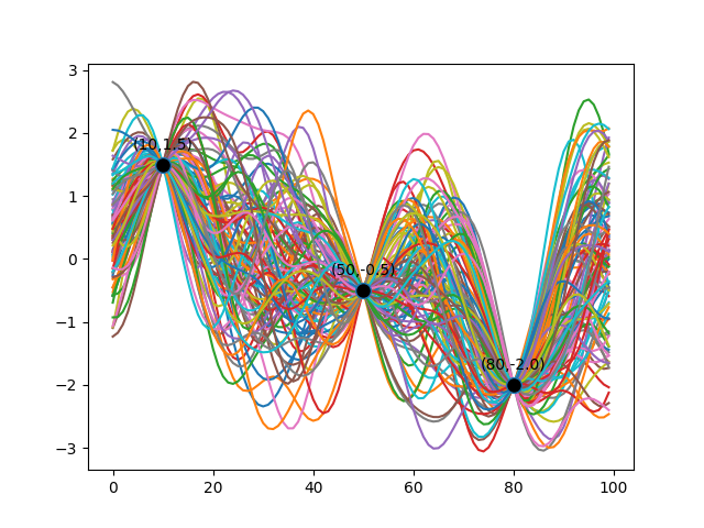
Recall the example Gaussian Process that we described in Gaussian Processes: Intuition. We demonstrated it by conditioning on three data points. The function distribution is reproduced below for reference.

Before there was any conditioning performed, the Gaussian Process was unbiased in terms of the functions it would pick, given the mean and the covariance matrix. Thus, the original covariance matrix (generated with a finite number of points) based on the exponentiated quadratic kernel looked uniform as below.

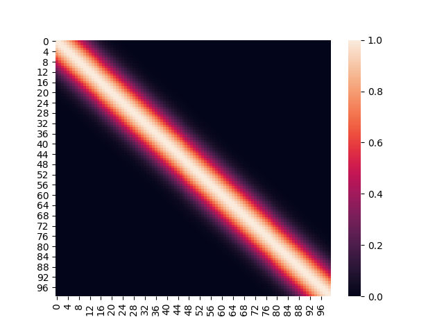
It is worth pointing out, that the middle white band represents input points which are closest to each other. The diagonal itself represents the covariance of a point with itself, essentially the variance.

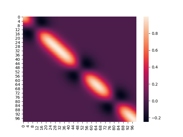
However, once we fix the three points, the covariance matrix starts to look a little different, like below.

If you notice the holes in the diagonal, they correspond directly to the indices (and the position) of the input points for which the distribution was conditioned. The variances at those points go to zero, because the values at those points has now been determined; hence the dark gaps in those positions of the covariance matrix.

Endnotes

There are a few topics that still need to be discussed in the context of kernels.

• Mercer Kernels
• Representation using Infinite Basis Functions
• Representer Theorem

These may be discussed in a future article.

---