Gaussian Processes: Intuition

Avishek Sen Gupta on 6 September 2021

---

In this article, we will build up our intuition of Gaussian Processes, and try to understand how it models uncertainty about data it has not encountered yet, while still being useful for regression. We will also see why the Covariance Matrix (and consequently, the Kernel) is a fundamental building block of our assumptions around the data we are trying to model.

To do this, we will cover the material in two phases.

The first pass (which is the focus of this article) will build the intuition necessary to understand Gaussian Processes and how they relate to regression, and how they model uncertainty during interpolation and extrapolation.

The second pass will delve into the mathematical underpinnings necessary to appreciate the technique more rigorously. This we will cover in a subsequent article.

The prerequisite for understanding this post is Geometry of the Multivariate Gaussian Distribution.

Function Sampling from Uncorrelated Gaussian Distributions

A Gaussian Process is capable of generating an infinite number of functions. The characteristics of these functions are wholly determined by the covariance matrix of this Multivariate Gaussian Distribution. Example characteristics that can be tweaked are how smooth (or how spiky) the functions are, whether they are periodic in nature or not, etc.

How are these functions generated? An important thing to keep in mind is that these functions do not have parametric forms, i.e., they do not take the form of familiar polynomials like \(x^2+3x+5\). Given the graph of a function (remember that graph represents the \((x,f(x))\) pairs of a function), each \(f(x)\) is generated by sampling from a Gaussian Distribution. This implies that if we are given a graph of \(N\) data points, we sample from a set of \(N\) Gaussian distributions.

Let us assume that the points given are indexed by \(\mathbb{N}\), so that the graph of the function looks like so:

\[1, \mathcal{N}_1(1) \\ 2, \mathcal{N}_2(2) \\ 3, \mathcal{N}_3(4) \\ \vdots \\ N, \mathcal{N}_N(N)\]

where \(\mathcal{N}_n\) represents an independent one-dimensional Gaussian distribution with some mean and variance.

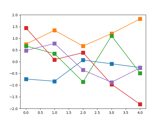
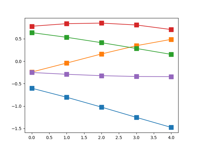
Now, this by itself doesn’t sound very bright. If we have a set of \(N\) independent Gaussians, and we sample once from each of them, we will get a set of \(N\) points, but there is no guarantee that it would be a “useful” function. The diagram below shows five such “functions” generated by sampling a set of five independent Gaussians \(\{\mathcal{N}_i\}_{i=1}^N\) (equivalently, an uncorrelated five-dimensional Multivariate Gaussian).

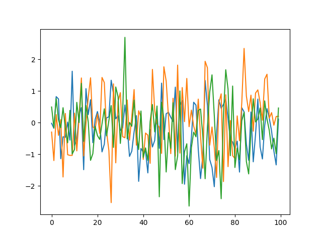
This is what the above would look like when the number of dimensions is increased.

Each run will generate a different function because \(\mathcal{N}_i(i)\) will return a (potentially) different value each time.

However, leaving aside the issue of smoothness for the moment, we have a way of generating a data set of \(N\) data points from \(N\) independent 1-D Gaussian distributions.

We can state the above in a different way: we can generate a data set of \(N\) data points by sampling an \(N\)-dimensional vector from an \(N\)-dimensional Multivariate Gaussian Distribution, all of whose random variables are independent of each other, i.e., are uncorrelated with each other.

Let me repeat: a single sampled vector from an \(N\)-dimensional Multivariate Gaussian represents one possible data set.

An \(N\)-dimensional Multivariate Gaussian is simply the product of \(N\) one-dimensional Gaussians, like so:

\[\mathcal{N}(X)=\prod\limits_{i=1}^N C_i\cdot \exp\left[-\frac{1}{2} \frac{ {(x_i-\mu_i)}^2}{\sigma_i^2}\right]\]

If you translate this into the canonical form of a Multivariate Gaussian Distribution, namely:

\[P(X)=K_0\cdot \exp\left( -\frac{1}{2} {(X-\mu)}^T\Sigma^{-1}(X-\mu)\right)\]

then the covariance matrix \(\Sigma\) is a diagonal matrix.

Smoother Functions and Correlated Gaussian Random Variables

Much of the data that we see in the real world is smooth, i.e., predictor values which are close to each other, yield predicted values which are also close to each other, not unlike the definition of continuity in Real Analysis.

The reason our generated functions in the previous section were spiky was because there was no modelling done to incorporate the idea of “smoothness” or “closeness” in our set of \(N\) Gaussian distributions.

This concept of closeness can be modelled by building correlations between the random variables. i.e., if the value of one random variable is high, there is a very high probability that the sampled value of the random variables near it are also high.

This correlation can be incorporated by modifying the covariance matrix \(\Sigma\) such that the random variables which are realised, are now correlated with each other. Note that this implies that the covariance matrix will now begin to have non-zero off-diagonal elements (it still remains necessarily symmetric).

Allowing correlated random variables in our Gaussian Process results in smooth functions. The covariance matrix represents how correlated each dimension is to each other.

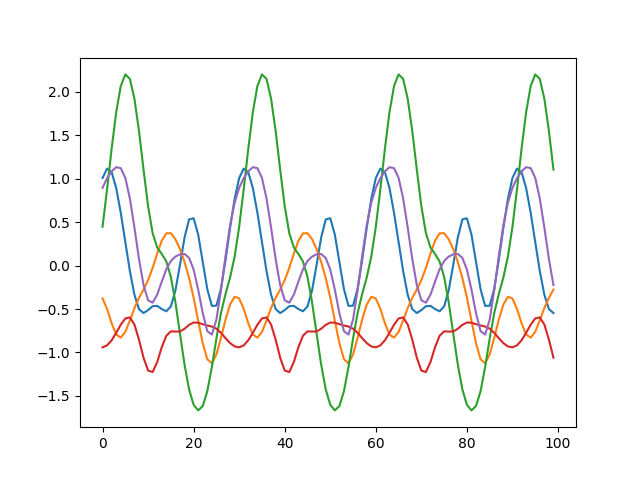
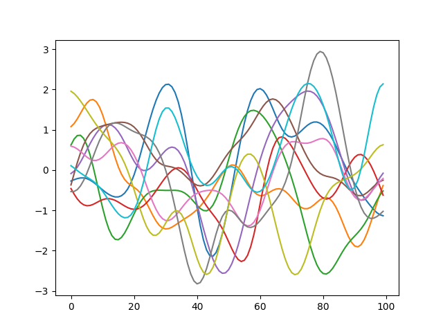
If the covariance matrix has correlations built in, sampling from the Gaussian Process results in functions like this (this specifically uses the exponentiated quadratic/RBF/Gaussian Kernel to calculate correlations, but we will have more to talk about this later).

Let us return to sampling our five-dimensional Multivariate Gaussian.None of its random variables are correlated with each other, which is equivalent to having a strictly diagonal covariance matrix. However, if we modify our covariance matrix to have non-zero off-diagonal elements, this becomes equivalent to building correlations between these random variables. The graph below shows five samples drawn from a \(\mathbb{R}^5\) Multivariate Gaussian with an exponentiated quadratic kernel (we will have more to say about kernels in a subsequent article).

You will notice that the spikiness that we saw in the uncorrelated version in the previous section is gone. This is because adjacent variables are correlated with each other. In fact, even variables farther apart are correlated, just not as strongly as the ones in their neighbourhood.

Increasing the number of dimensions of our correlated Multivariate Gaussian gives us functions which are “smooth”. Effectively, if you have an infinite covariance matrix, then you have a corresponding infinite-dimensional Multivariate Gaussian Distribution which can generate a function (remember that a function is essentially an infinite-dimensional vector) which would be defined for every possible value of its parameter, i.e., the set of indices become \(\mathbb{R}\).

Incorporating Training Data and Conditioning

Now we have access to an infinite set of smooth functions from a (potentially infinite-dimensional) Multivariate Gaussian. Our problem now boils down to this: given a set of training data, we’d like to select the subset of functions which pass through the training data.

At this point, our infinite set of functions have no constraints imposed on them. The constraint we wish to apply is that any candidate function for regression must pass through the set of points in our training data.

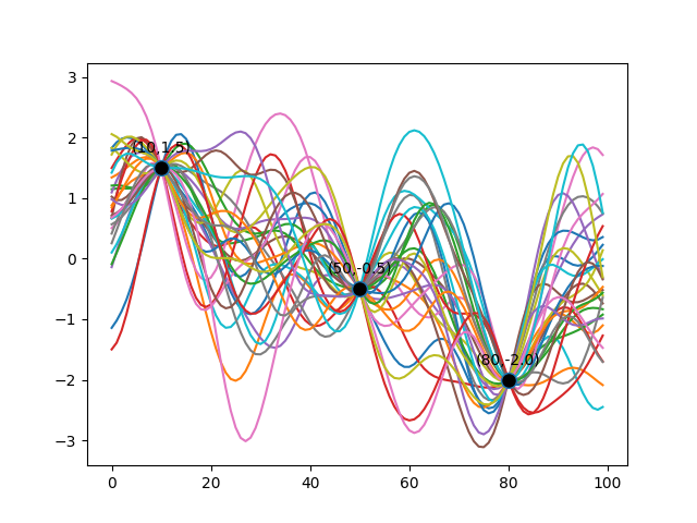
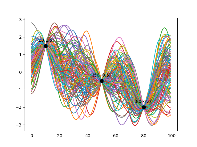
Once we clamp the Multivariate Gaussian at certain points, sampling the resulting Multivariate Gaussian Distribution gives us something like the following diagram. Here, I’ve chosen three arbitrary training data points to illustrate that the subset of functions we pick, all pass through these training data.

The diagram below shows 100 functions sampled from a 100-dimensional Multivariate Gaussian.

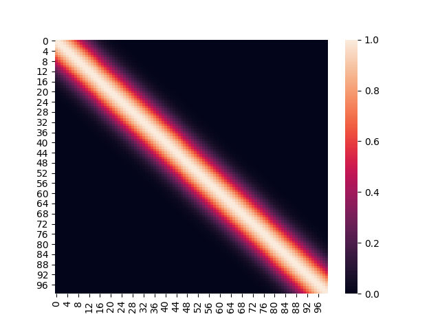
The initial covariance matrix (using the exponentiated quadratic kernel) looked like this:

After incorporating training data, the covariance matrix looks like so:

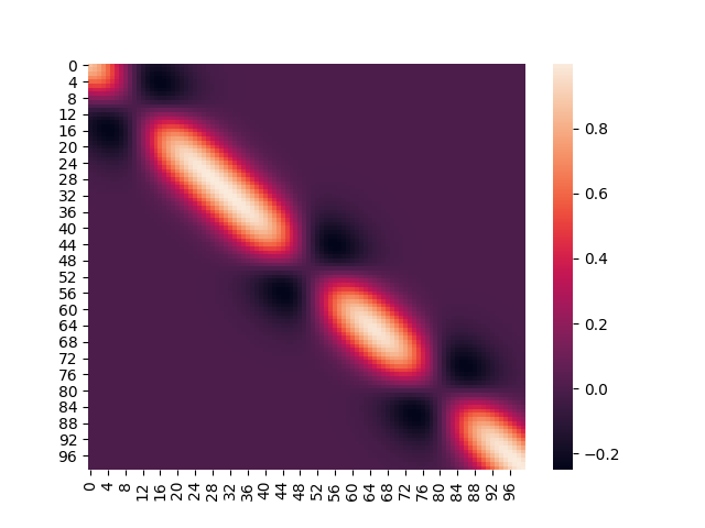
We will discuss how this difference comes about in an upcoming article.

Modelling Uncertainty

As it is evident, all the functions that we select (how we does is addressed in the Mathematical Underpinnings section) pass through our training data. You will also have noticed that those functions assume a range of values for all points between our training data points. This is how uncertainty is modelled in Gaussian Processes: the range of variation outside of our training data, represents our uncertainty about what data could feasibly reside in those regions.

This is the crux of how Gaussian Processes work.

• A (potentially infinite-dimensional) Multivariate Gaussian Distribution with a Covariance Matrix (defined using a problem-specific Kernel) is the source of an infinite number of functions.
• The characteristics of these functions is controlled by the nature of Kernel.
• A single sample from this Multivariate Gaussian represents an entire function (an infinite-dimensional vector).
• We select a subset of these functions which are constrained to pass through our training data.
• The regions between (and outside) our training data represent our uncertainty about what data exists in those regions.
• Conditioning a Multivariate Gaussian distribution is equivalent to setting a specific dimension to a specific value (which is usually a point in the test data set).

Kernels and Modelling Domain Knowledge

An important question usually arises during the construction of the covariance matrix, namely, how do we measure the similarity between two points? Using the normal inner product approach is one answer, but it is not the only answer.

If you remember the discussion around Inner Product in Kernel Functions: Functional Analysis and Linear Algebra Preliminaries, any function which satisfies the following properties, can serve as a measure of similarity.

• Positive Definite: \(\langle x,x\rangle>0\) if \(x\neq 0\)
• Principle of Indiscernibles: \(x=0\) if \(\langle x,x\rangle=0\)
• Symmetric: \(\langle x,y\rangle=\langle y,x\rangle\)
• Linear:
  • \[\langle \alpha x,y\rangle=\alpha\langle x,y\rangle, \alpha\in\mathbb{R}\]
  • \[\langle x+y,z\rangle=\langle x,z\rangle+\langle y,z\rangle\]

Accordingly, a variety of functions can serve as measures of similarity: these are commonly referred to as kernels, and they are the same kernels that we have discussed while talking about the construction of Reproducing Kernel Hilbert Spaces in Kernel Functions with Reproducing Kernel Hilbert Spaces.

The important thing to note is that the choice of kernel in a Gaussian Process is a modelling decision that a domain expert can take, to incorporate prior knowledge of the domain into the prediction process. In this manner, domain knowledge can be exploited while setting up a Gaussian Process for Machine Learning.

We will briefly consider two kernels. There may be more material on combining kernels to create new ones, in a future article.

1. Radial Basis Function Kernel

We have also encountered this kernel: we have simply referred to it as the Exponentiated Quadratic Kernel. It is essentially a Gaussian pressed into service to measure similarity between two points. The covariance matrix formed from such a kernel, looks like the image below.

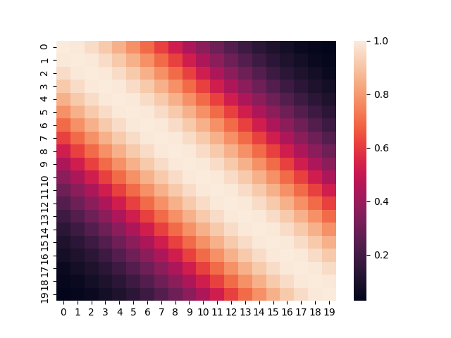
The expression for the RBF Kernel is obviously a Gaussian.

\[K(x,y)=K\cdot \exp\left(-\frac{1}{2}\frac{ {(x-y)}^2}{\sigma^2}\right)\]

We have already encountered the types of functions that can be sampled based on this kernel.

2. Periodic Kernel

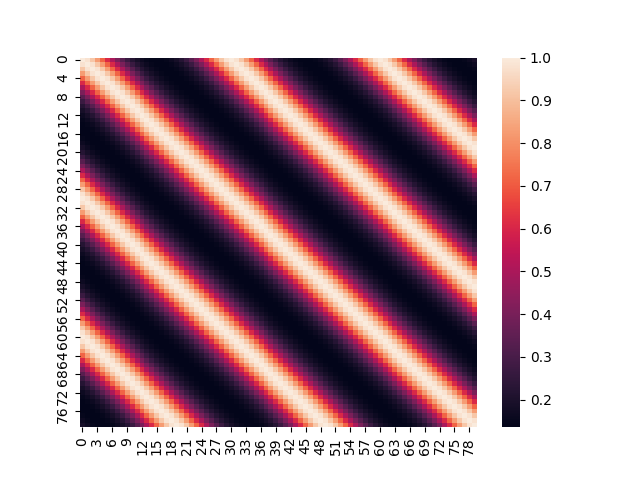
The Periodic Kernel, as its name suggests, can be used to model variations which are potentially periodic in nature. Its expression looks like so:

\[K(x,y)=\sigma^2\exp\left[-\frac{2}{l^2}\cdot \text{sin}^2\left(\pi\frac{\|x-y\|}{p}\right)\right]\]

An example covariance matrix based on a Periodic Kernel, looks like this:

Sampling a Multivariate Gaussian with a covariance matrix built based on the Periodic Kernel, yields functions like the following:

---