Background: This post took me a while to write: much of this is motivated by problems that I’ve noticed teams facing day-to-day at work. To be clear, this post does not offer a solution; only some thoughts, and maybe a path forward in aligning developers’ and architects’ thinking more closely with the frameworks used by people controlling the purse-strings of software development projects.
The posts in this series of Software Engineering Economics are, in order:
- Every Software Engineer is an Economist (this one)
- Every Software Engineer is an Accountant
- Economic Factors in Software Architectural Decisions
[WIP] Here is a presentation version of this article.
The other caveat is that even though this article touches the topic of estimation, it is to talk about building uncertainty into estimates as a way to communicate risk and uncertainties with stakeholders, and not to refine estimates. I won’t be extolling the virtues or limitations of #NoEstimates, for example (sidebar: the smoothest teams I’ve worked with essentially dispensed with estimation, but they also had excellent stakeholders).
“All models are wrong, but some are useful.” - George Box
Every software engineer is an economist; an architect, even more so. There is a wealth of literature around articulating value of software development, and in fact, several agile development principles embody some of these, but I see two issues in my day-to-day interactions with software engineers and architects.
- Folks are reluctant to quantify things they build, beyond the standard practices they have been brought up on (like basic estimation exercises, test coverage). Some of this can be attributed to their prior bad experiences of being micromanaged via largely meaningless metrics.
- Folks struggle to articulate value beyond a certain point to stakeholders who demand a certain measure of rigour and/or quantifiability. Similarly, engineers fail to communicate risk to decision-makers. The problem is then that The DORA metrics are good starter indicators, but I contend that they are not enough. Let me be as clear as possible: CxOs don’t really care about precious developer metrics; they really care about the savings or profits which result from improving those metrics.
- There is a reluctance to rely too much on metrics because people think metrics are easily gamed. This can be avoided if we use econometric methods, because 1) falsified data is immediately apparent 2) showing the work steps, assumptions and risks aids in this transparency because they are in the language of economics which is much more easily understandable to business stakeholders.
- Thinking about value and deciding tradeoffs based on economic factors is not something that is done enough, if at all, at the level of engineering teams. For example, questions like “Should I do this refactoring?” and “Why should we repay this tech debt?”, or “How are we better at this versus our competitor?” are usually framed in terms of statements which stop before traversing the full utility tree of value.
Thinking in these terms, and projecting these decisions in these terms to managers, heads/directors of engineering – but most importantly, to execs – is key to engineers articulating value in a manner which is compelling, and eases friction between engineering and executive management. It is also a skill engineers should acquire and practise to break several firms’ perceptions that “engineers are here to do what we say”.
This is easier said than done, because of several factors:
- The data to apply these frameworks is not always easily available, and may require additional investment.
- Engineers can get invested in decisions that they think are their “pet” ideas.
- It can be hard to inculcate this mindset en masse among engineers if they do not have a clear perception of the value of adopting this mindset. Engineers don’t want theory, they want tools they can apply quickly and easily. Hence, the burden is on us to propose advances to the state of the art in a way that is actionable.
Most of the thinking and tools discussed in this article have been borrowed from domain of financial engineering and economics. None of this material is new; a lot of research has been done in quantifying the value of software-related activities. The problem usually is translating those ideas into actions.
For these ideas to effectively work, they must permeate all the way across developers to tech leads to architects to managers. Thus, this article is divided into the following sections:
- Communicating Uncertainty and Risk in Estimation Models
- Articulating the Value of Timing (aka, Real Options)
- Communicating Values and Risks of Tech Debt and Architectural Decisions
- Deriving Value in Legacy Modernisation
- Articulating the Value of Measurement (aka, the Cost of Information)
Simplifying Assumptions
- The conversion of time to money is simply treated as the Cost to Company for a single individual working. This is a lower bound, since there will usually be multiple people on a work item, and there may be other ancillary costs.
Key Concepts
1. Net Present Value and Discounted Cash Flow
The concept behind the Time Value of Money is to calibrate some amount of money in the future to the present value of money. The idea is that a certain amount of money today is worth more in the future. This is because this money can be invested at some rate of return, which gives you returns in the future. Hence, receiving money earlier is better than receiving it late (because you can invest it right now). Similarly, spending money later is better than spending it right now, because that unspent money can earn interest. If \(r\) is the rate of return (sometimes also called the hurdle rate), then \(P_0\) (the amount of money right now) and the equivalent amount of money \(P_t\) after \(t\) time periods are related as:
\[P_0=\frac{P_t}{ {(1+r)}^t }\]When making an investment, there are always projections of cash inflows and outflows upto some time in the future, in order to determine whether the investment is worth it. The sum of all of these cash flows (corrected to Net Present Values) minus the investment is a deciding factor of whether the investment was worth it; this is the Discounted Cash Flow, and is written as:
\[DCF(T)=\sum_{t=1}^T \frac{ CF(t)}{ {(1+r)}^t }\]where \(CF(t)\) is the cash flow at period \(t\), and \(r\) is the rate of return. Subtracting the investment from this value gives us the Net Present Value. If the NPV is positive, the investment is considered worth making, otherwise not.
2. Financial Derivative and Call Options
A Financial Derivative is a financial instrument (something which can be bought and sold) whose price depends upon the price some underlying financial object (henceforth called “underlying”). For simplification, assume that this underlying is a stock. Thus the price of a derivative depends upon the price of the stock.
A Call Option is a kind of financial derivative. There are different kinds of call options; for the purposes of this discussion, we will discuss American Call Options, and simply refer to it henceforth as “option”. The following are the characteristics of a call option (options in general, in fact):
- The option is associated with a specific stock.
- The option costs money to buy. This is called the Option Premium. This is almost always less than the price of the underlying stock.
- The option has an expiry date.
- The option can be exercised at any time before its expiry date.
- The option has a strike price, which is fixed at the time of purchase of the option. If the option owner exercises the option, they can buy the underlying stock at the strike price, regardless of the price of the stock at that time on the financial market.
The idea is that we can pay a (relatively) small amount to fix the price of the stock for the lifetime of the option. If we choose to never exercise the option, the option lapses, and we have incurred a loss (because we paid for the option premium).
- Let’s take a simple example. The current stock price is $100. Let there be an option to buy this stock, with a strike price of $100. The option premium is $10.
- We buy one option, and thus pay $10.
- A few days later, the stock price rises to $120. We exercise the option, and buy the stock for $100, which is the strike price. We pay $100. We have paid a total of $110 so far.
- We immediately sell the stock to the market at the current stock price of $120.
- We have thus earned $120-$110=$10.
Thus, options allow us to speculate on rising stocks. It is worth noting that there is the counterpart to the Call Option, which is the Put Option, which gives us the option to sell a stock at the specified strike price.
1. Articulating Value: Communicating Uncertainty and Risk in Estimation Models
Scenario: The team is asked to estimate a certain piece of work. The developers and analysts put together the usual RAIDs (Risks, Assumptions, Issues, Dependencies), and come up with a number (or, if they are slightly more sophisticated, they throw a minimum, most likely, and maximum value for each story). They end up adding up the maximum values to get an “upper bound”, do the same thing to the other two sets of estimates to get a total lower bound, and a total likely estimate. The analyst or the manager goes “This is too high!”. The developers go back to their estimates and start scrutinising the estimates, all in the hope of finding something they can reduce. Most of the time, they simply end up lowering some estimates (by fiat, or common agreement); this may be accompanied by a rational explanation or not: the latter is usually more common.
Happy with this number, the manager marches off to the client and shows off this estimate. The budget is approved; work commences. Then along comes the client all indignant: “We are not meeting the sprint commitments! The team is not moving fast enough!” Negotiations follow. No side ends up happy.
There are so many things wrong in the above picture; unfortunately, this can happen more often than not. What has happened here is a failure of communication; between the developers and the manager, and between the team and the client. One of the primary reasons for this is the false sense of accuracy and precision that comes with ending up with a single number, and the lack of tools to articulate the uncertainty behind this number. What does “upper bound” mean? Are you saying it will never go past this number?
If there is a clear way of communicating this uncertainty, the team can make an informed decision of what level of risk they are taking up when committing to a certain estimate. The client would certainly appreciate this, instead of receiving a single number which ends up being treated as an ironclad guarantee of the date of delivery.
Thankfully, we can communicate this uncertainty using some time-tested statistical tools.
Estimation Procedure using Confidence Levels
- We assume that the estimate of a story is normally distributed. A potentially better candidate could be the log normal distribution, but let’s keep it simple for now.
- When you throw an estimate, pick a range. This range is not simply an “upper bound” and “lower bound”, but it answers the question: “I’m 90% certain that it falls within \(x\) and \(y\)“. We don’t bother with the most likely estimate in this scenario (it might matter if we are using something other than a Gaussian distribution, but let’s keep it simple).
- Calculate the variance \(\sigma\) given confidence interval of 0.9 (Z-score is correspondingly 1.65). Note that Confidence Interval is defined as \(\hat{X} \pm Z.\sigma\).
- Do this for each story.
- Calculate the joint probability distribution of all the random variables (one per story). This is easy if we assume all the estimate distributions are Gaussian. If not, perform Monte Carlo simulations. This will give you a new normal distribution that represents the aggregate of all your estimate distributions.
- Pick a range of estimates based on an acceptable confidence level. Alternatively, pick an acceptable range of estimates, record the confidence level, and acknowledge the risk. Communicate this range and the confidence with the client.
- Negotiation with the client (or within the team) should happen around acceptable levels of uncertainty levels, not on modifying story estimates to fit a particular target. As long as all parties acknowledge the risk level, the uncertainty is explicitly communicated and may preempt the client coming back disappointed because the recorded effort exceeded a single number.
See this spreadsheet for a sample calculation. In the diagram below, the normal distribution on the far right is the final distribution resulting from convolving all the story estimates (which are normal distributions themselves). The Y-axis has been scaled by 1000 for ease of visualisation.
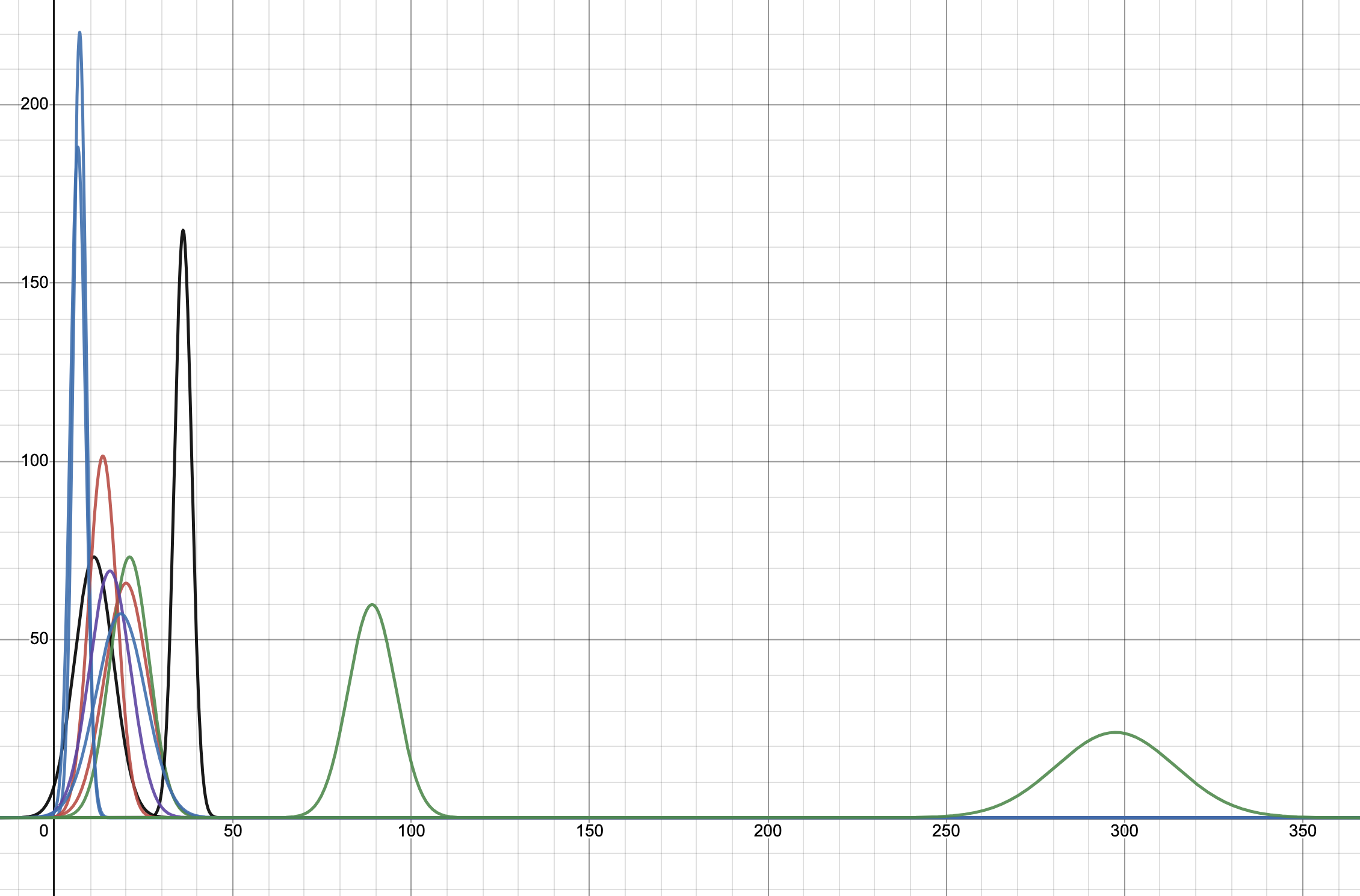
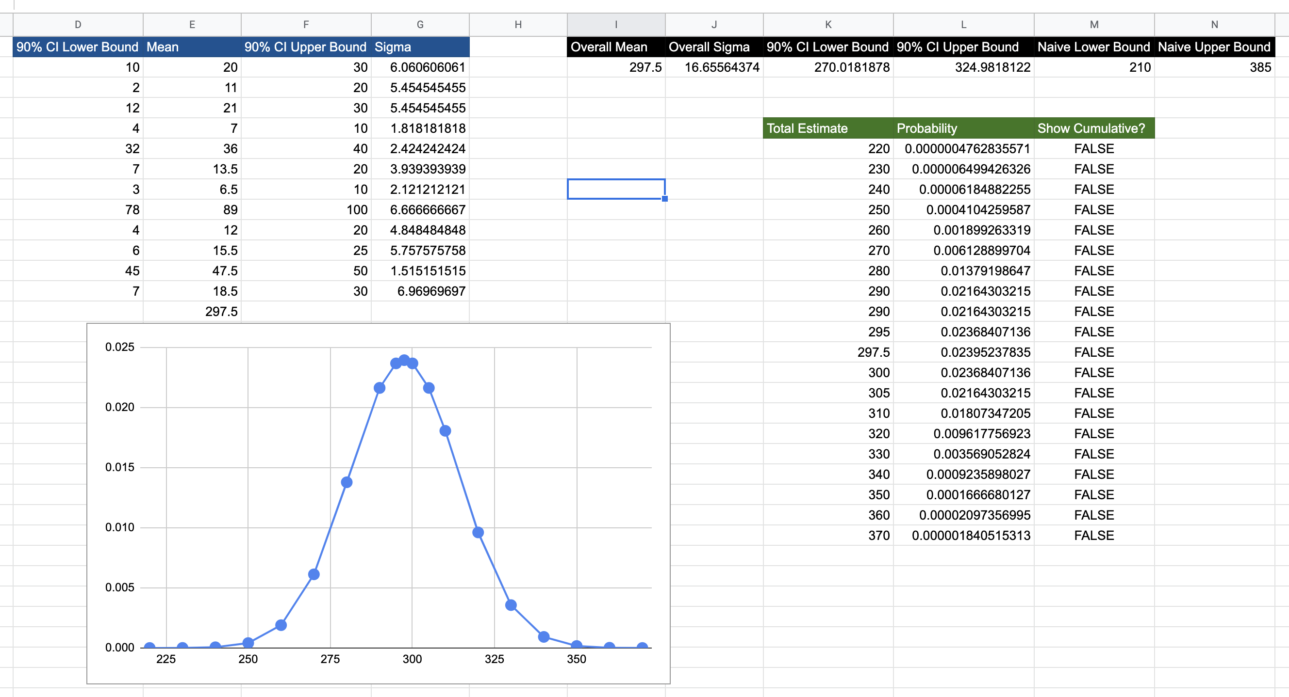
As you can see, the attempt to find a naive lower and upper bounds by summing the lower and upper bounds gives us 210 and 385. In fact, it is misleading to call these simply lower and upper bounds. They are bounds, but in this case, we want to use the term 90% confidence level upper/lower bounds. This implies that the estimators are 90% sure that the estimates for the first story (for example) lies between 10 and 30. Using this metric and using proper convolution techniques yields these bounds as 270 and 324, which is different from the value of naive summation, and is the correct result. With more stories, the gap between the convolution approach and the naive summation increases. One point about the 90% confidence level: whether narrowing this uncertainty is worth it (without artificially manipulating numbers) is the subject of the discussion in Articulating Value: The Value of Measurement. However, the point is to not settle on a single number, but to always use a range of values. This, in itself, is not new. However, the upper and lower bounds are always taken as fixed, without any discussion around the risk involved in picking a lower estimate.
This is what the above calculation brings out. In this simplifying example, we have chosen the estimates to be normal distributions, to keep calculations simply. It could even be a fat-tailed distribution like a Log-Normal Distribution (to bias it towards higher estimates), but then we’d need to run Monte Carlo simulations to come up with the data. So, let’s keep it simple for now.
The correct approach of convolving the estimate sdistributions of all the stories results in the single normal distribution above. With this graph, we can answer questions like:
- What are the upper and lower bounds with 90% confidence? 324 and 270, respectively, which is different from the result of naively summing the upper and lower bounds.
- Suppose we want to use a lower estimate of the upper bound, say, 310; what then is the risk of being wrong? The answer is 23%, which you can calculate for yourself by going to the spreadsheet directly.
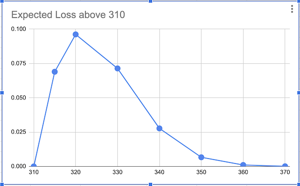
The idea is that you can now communicate risk in your estimates, in the form of risk exposure. This is done by finding the expected differential between your upper bound and the overshoot value of the normal distribution from the probability at the upper bound to \(\infty\). In this case, risk exposure communicates how much extra time (and consequently, money) will need to be expended, if the estimate overshoots 310 (assuming the budget was allotted only for 310).
The risk exposure curve for the above scenario is shown below:
Interesting Note: The IEEE-CS/ACM Software Engineering Code of Ethics and Professional Practices requires software professionals to quote uncertainties along with their estimates.
2. Articulating Value: The Value of Timing (aka, Real Options)
Real Options
Competent Architects and Engineers identify Real Options. Good Architects and Engineers create Real Options.
We have already talked about options earlier. Here we talk about Real Options, which are the strategic equivalent of Call Options. Most of the characteristics remain the same; however, real options are not traded on financial markets, but are used as a tool to optimise investments. We will delve into some of its possible applications in architectural decision-making and technical debt repayment, by way of example. Specifically, the YAGNI principle derives from the Real Options approach. See the following references for excellent discussions on the topic:
- Software Design Decisions as Real Options
- The Software Architect Elevator
- Chapter 4 of Extreme Programming Perspectives
- Chapter 3 of Value-Based Software Engineering
Here is an example. Let us assume that we have an Architecture Decision that we’d like to implement. The investment to implement this is 70. We project the following probabilities:
- 30% chance that the change will result in savings of 45 (in the current legacy process) per month for the next 3 months
- 40% chance that the change will result in savings of 30 (in the current legacy process) per month for the next 3 months
- 30% chance that the change will result in savings of 15 (in the current legacy process) per month for the next 3 months
Furthermore, we have determined that the Risk-Free Rate of Interest and the Risk Interest Rate are 6% and 10%, respectively. These will be used to calculate the Discounted Cash Flows.
The two scenarios are presented in this spreadsheet.
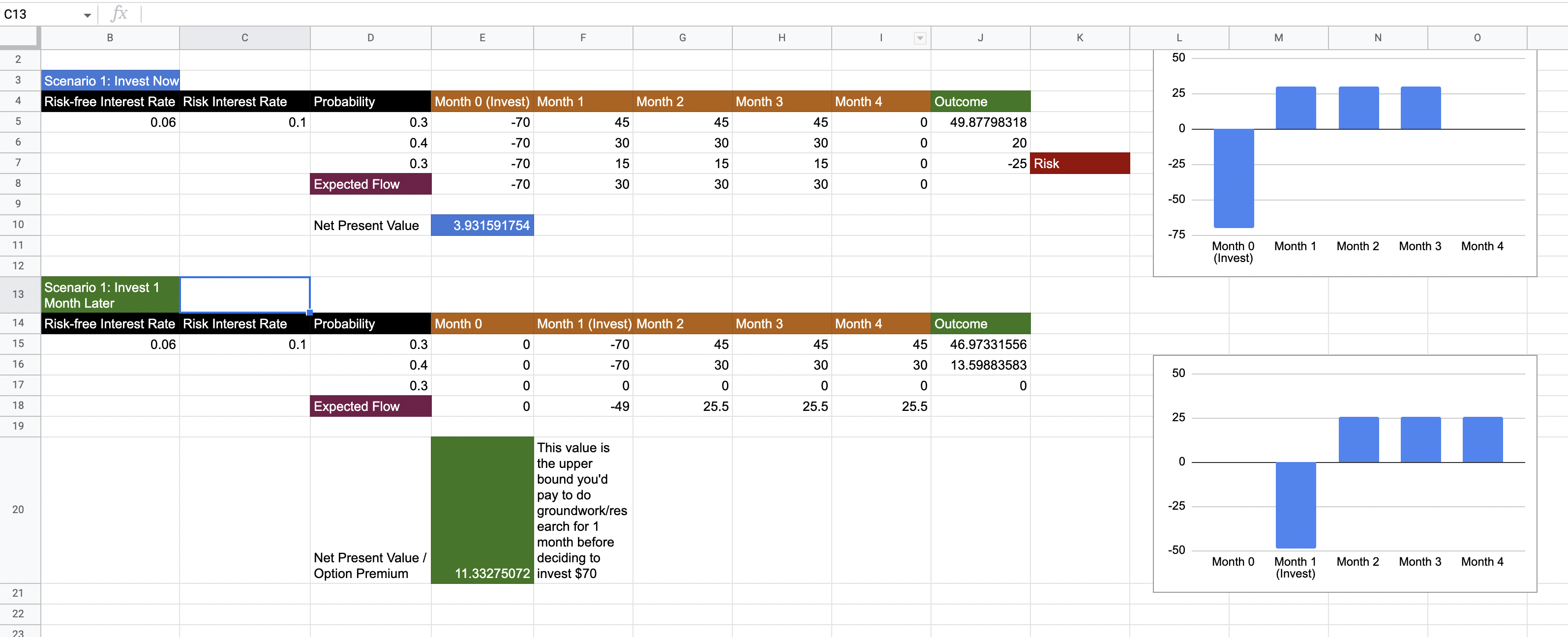
We see that the Expected Net Present Value is 3.9. This is a positive cash flow, so we might be tempted to implement the architecture decision right now. However, consider the risk. There is a 30% chance that the investment will be more than the savings and that we will end up with a negative cash flow of 25.
Let us assume that we wait a month to gather more data or more importantly, run a spike to validate that this architecture will pan out to give us the desired savings. How much should we invest into the spike? Usually, spikes are timeboxed, but for larger architecture decisions, we can also put a economic upper bound on investment we want to make in the spike.
The second set of calculations above show the second scenario of waiting a month. We see that if we can eliminate the uncertainty of incurring a loss (i.e., the [30%,15] scenario), the Net Present Value of the endeavour comes to 11.33. This is much higher than the NPV of the first scenario. This implies that waiting for one month doing the spike, and then making a decision is more valuable.
More importantly, this value of 11.33 gives us the Option Premium, which is the maximum value we’d like to pay in order to eliminate this uncertainty of loss. Note that this number is much less than the investment we’d have to make. Essentially, we are paying the price of eliminating uncertainty, and we’d like to make sure that this price is not too high.
Incidentally, the above calculations use the Datar-Matthews, because its parameters are more easily estimatable, but it also gives the same results as the famous Black-Scholes Model, which is used to price derivatives in financial markets.
Examples
- One example where we could have applied: The team had built a data engineering pipeline using Spark and Scala. The stakeholder felt that hiring developers with the requisite skillsets would be hard, and wanted to move to plain Java-based processing. A combination of cash flow modeling and buying the option of redesign would have probably made for a compelling case.
So, to reiterate: real options are valuable because they allow us to make smaller investments to eliminate uncertainty on the return on investment for a large investment, without actually making that investment immediately, but deferring it. The value comes from deciding whether to defer this investment or not, whether this investment is implementing an architectural decision, or repaying tech debt. In many situations, the Real Option Premium is effectively zero, which means we don’t really need to do anything, but can just wait for more information on whether the investment seems worthwhile or not.
More philosophically, every line of code we write is an investment that we are making right now: an investment which might be worth delaying. Articulating this value concretely between engineers grounds a lot of discussions on what is really valuable to stakeholders, and will preempt a lot of bike-shedding.
3. Articulating Value: Economics and Risks of Tech Debt and Architectural Decisions
Here is some research relating Development Metrics to Wasted Development Time:
- Code Red: The Business Impact of Code Quality - A Quantitative Study of 39 Proprietary Production Codebases
- The financial aspect of managing technical debt: A systematic literature review
- The Pricey Bill of Technical Debt: When and by Whom will it be Paid?
ATD must have cost=principal (amount to pay to implement) + interest (continuing incurred costs of not implementing ATD)
The following is an example of how a cash flow of an architectural decision might look like.
graph LR;
architecture_decision[Architecture Decision]-->atd_principal[Cost of Architectural Decision: Principal];
architecture_decision-->recurring_atd_interest[Recurring Costs: Interest];
architecture_decision-->recurring_atd_savings[Recurring Development Savings];
architecture_decision-->atd_option_premium[Architecture Option Premium];

style architecture_decision fill:#006fff,stroke:#000,stroke-width:2px,color:#fff
Incorporating economics into daily architectural thinking
Here are some generic tips.
- Practise drawing causal graphs. Complete the trace all the way up to where the perceived benefit is (money) is. It may be tempting to stop if you reach a DORA metric. Don’t; get to the money.
- If you are already measuring DORA metrics, relentlessly ask what each DORA metric translates to in terms of money.
- Along the way of the graph, list out other incidental cash outflows.
- Build an option tree. Deduce whether it is better to defer execution, or do it right now. See Articulating Value (The Value of Timing, aka Real Options) for guidance on this.
- Examples of architectural options are (see Articulating Value: The Value of Timing):
- Architecture Seams in Monoliths
- Spikes
- Simply waiting (YAGNI - You Aren’t Gonna Need It)
- Non-technical things can also be calculated, i.e., the need for training.
- These metrics must be measured as part of standardised project protocols.
Here are some tips for specific but standard cases.
1. The Economics of Microservices
If you are suggesting a new microservice for processing payments, these might be the new cash flows, as an example:
- Recurring Cash Flows
- Transactions: New cash inflow
- Cost of recovering the whole system back from failure: Reduced cash outflow
- Cost of cloud resources to scale the new microservice: New cash outflow
- Cost of higher latency leading to lower service capacity (if the microservice is part of a workflow): Decreased cash inflow, depending upon if you ever reach the load limits of the service before other parts of the system start to fail
- Cost of fixing bugs: New cash outflow, depending upon complexity of the microservice
- Cost of Integrations:
- Single or Few-Time Cash Flows
- Cost of development: New cash outflow
- Cost of deployment setup: New cash outflow (ideally should be as low as possible)
- Option Premium
- Architecture Seam (see Articulating Value: The Value of Timing)
graph LR;
microservice[Microservice ADR]-->database[Cloud DB Resources];
microservice-->hosting[Cloud Hosting Resources];
microservice-->development_cost[Development Cost];
microservice-->latency[Latency];
microservice-->bugs[Fixing bugs]-->bugfix_time[Wasted Bugfix Time Costs];
microservice-->downtime[Downtime]-->lost_transactions[Lost Transaction Costs];
microservice-->microservice_option_premium[Architecture Seam: Option Premium];

style microservice fill:#8f0f00,stroke:#000,stroke-width:2px,color:#fff
2. The Economics of Technical Debt repayment
- Recurring Cash Flows
- Cost of Manual Troubleshooting and Resolution
- Cost of recurring change to a specific module
- Single or Few-Time Cash Flows
- Cost of repaying tech debt
- Option Premium
- The cost of isolating the effect of the technical debt from affecting other code (see Articulating Value: The Value of Timing)
The following is an example of how a value tree of a (general) Tech Debt might look like.
graph LR;
debt[Tech Debt]-->principal[Cost of Fixing Debt: Principal];
debt-->interest[Recurring Cost: Interest];
debt-->td_option_premium[Tech Debt Option Premium];
debt-->risk[Risk-Related Cost, eg, Security Breach];

style debt fill:#006f00,stroke:#000,stroke-width:2px,color:#fff
Example Tech Debt Cash Flow
We see options thinking happening on projects to some degree; however they are either not explicitly articulated, nor are the value of these decisions explicitly communicated to stakeholders. This is corroborated in the paper How Do Real Options Concepts Fit in Agile Requirements Engineering?, where they attempt to answer some research questions. The ones of interest are listed below, and the relevant excerpts are quoted from this paper.
Research Question: What is the level of agile software organizations’ awareness of using options thinking in support of agile requirements reprioritization?
“Both the literature sources and the case study showed that there is awareness in the organizations, and that they apply option thinking for making mid-course project decisions, both from clients and developers perspective. Although the agile companies propagate development process driven only by value creation for the client, we observed that in practice option thinking is intrinsic for the developers as well. They consider trade offs between quality and schedule…”
Research Question: In which way does options-thinking add value?
” In the searched literature, we could not find a case where options are explicitly documented and compared in terms of value or in other quantitative way.”
Research Question: Which aspects of using options thinking in agile RE can be recognized as topics for future research?
“…we found that the options thinking is mostly described in terms of how it works for developers’ organizations. The perspective of the clients’ organizations seems under-researched.”
“We must note that in the literature, we found instances of using options-thinking which represent anecdotic experiences of either agile consultants or agile-practiceadopting organizations. We were really surprised that we couldn’t find a more substantive evidence that could be used to answer our research questions.”
“In both the literature review and the case study, we found that options are not expressed in quantitative terms. This finding makes us think that it may not be realistic at all to expect agile teams to reason about options quantitatively. Whether this is the case or not is a line for future research.”
(I emphatically contend that quantification of value in concrete economic terms should be one of the building blocks of articulating this value.)
4. Articulating Value: Deriving Value in Legacy Modernisation
Legacy Modernisation is an involved beast, and usually there are far too many variables to create an exhaustive model. However, a candidate cost model is a starter. We’ll write more about this going forward.
\(C_{HW}\) = Cost of Hardware / Hosting
\(C_{HUF}\) = Cost of manual work equivalent of feature (if completely new feature or if feature has manual interventions)
\(C_{RED}\) = Cost of recovery, including human investments (related to MTTR)
\(C_{LBD}\) = Cost of lost business / productivity during downtime (related to MTTR)
\(C_{ENF}\) = Cost of development of an enhancement to a feature (related to DORA Lead Time)
\(C_{NUF}\) = Cost of development of a new feature (related to DORA Lead Time)
\(C_{BUG}\) = Cost of bug fixes for feature
\(n_D\) = Number of downtime incidents per year
\(n_E\) = Number of enhancements to feature per year
\(n_B\) = Number of bugs in feature per year
The cost of a feature is then denoted by \(V\), and the total value of the feature is \(V_{total}\). These are given by:
\[V=C_{HUF} + n_D.(C_{RED} + C_{LBD}) + n_E.C_{ENF} + n_B.C_{BUG} \\ V_{legacy} = \sum_{i} V_i + C_{HW} + n_F.C_{NUF}\]In legacy modernisation, the idea is to minimise \(V_{legacy}\), so that \(V_{legacy}-V_{modern} > 0\). Retention of customer base is also a valid use case, which we will touch upon in sequels.
5. Articulating Value: The Value of Metrics (aka, the Cost of Information)
For a metric to have economic value, it must support a decision. Examples of decisions are:
- The investment will either be made or not. Alternatively, the amount of investment will be more or less.
- Teams will be restructured or not.
- A feature will go live or not.
- A system (or subsystem) will be modernised or not.
- A system will be either bought or built in-house.
Characteristics of a Decision
- Must have 2 or more realistic alternatives. These alternatives cannot be recursive, i.e., the decision based on a certain measurement should not be to take action to modify that measurement.
- A decision has uncertainty.
- A decision has potentially negative consequences.
- A decision must have a decision maker.
Quantify the Decision Model. The Decision Model will probably have multiple variables.
We need to decide what is the importance of these variables in making the decision. If a measurement has zero information value, then it is not worth measuring. When multiple variables are involved, use the EVPI metric coupled with Monte Carlo simulations (assuming the decision model has been quantified) to decide on the most important metrics.
Before we get into the nitty-gritties of how to actually measure this, let’s talk about the chain of value where we trace a metric to its value to the business decision it facilitates.
In general, any metric’s value tree should encapsulate (most of) the following elements.
graph LR;
metric[Metric]-->speed[Speed]-->time_to_market[Time to Market]-->first_mover_fast_follower[First Mover/Fast Follower Economic Advantage]
time_to_market-->time_value[Time Value of Savings/Profits]
first_mover_fast_follower-->|No|no_invest[Don't Invest]
first_mover_fast_follower-->|Yes|invest[Invest]
time_value-->|Low|less_invest[Invest Less]
time_value-->|High|more_invest[Invest More]
It is also important to note that a single metric does not contribute to the speed effect. Other factors like development effort are key input factors in custom software development. Let’s speak of the values which a metric can be traced to.
- First Mover/Fast Follower Economic Advantage: The advantage gained by getting to market first with a novel product or feature is not to be underestimated. This is the First Mover Advantage. However, the First Mover Advantage has been disputed with the proposition that the Second Mover / Fast Follower Advantage may be significantly less riskier, and as profitable, if note more. Regardless of debate in this area, speed plays a key contribution in gaining this advantage.
- Time Value of Savings/Profits: The value of speed not only lies in a first mover advantage. Even if we discount such an advantage, we can see that a savings (or profit) made earlier is always more valuable than the same amount gained at a later point in time, as we noted in Key Concepts. Essentially, the later the client starts seeing the profits/savings, the more money they are losing. At the risk of repeating the concept, this is because the savings or profits made right now could be invested and gaining returns from that interest.
The Economics of DORA Metrics
What business decisions do DORA metrics support? We can follow the above value tree, and see that they fit in very well with the template.
- Deployment Frequency is a proxy for speed of feature development, which is itself a proxy for time to market.
- Lead Time for Changes is a proxy for speed of feature development, which is itself a proxy for time to market.
- Mean Time to Recovery is a metric for financial loss during downtime.
- Change Failure Rate is a proxy for speed of development of features, which is itself a proxy for time to market.
This is an example value tree for DORA metrics.
graph LR;
df[Deployment Frequency]-->speed[Speed]-->time_to_market[Time to Market]-->first_mover_fast_follower[First Mover/Fast Follower Economic Advantage]
mlt[Lead Time for Changes]-->speed
cfl[Change Failure Rate]-->bugs[Bugs]-->speed
time_to_market-->time_value[Time Value of Savings/Profits]
first_mover_fast_follower-->|No|no_invest[Don't Invest]
first_mover_fast_follower-->|Yes|invest[Invest]
time_value-->|Low|less_invest[Invest Less]
time_value-->|High|more_invest[Invest More]
There are a lot more concepts that I’d like to cover, including:
- Expected Value of Perfect Information
- Possible procedures for determining the value of a metric
- When is a metric’s performance good enough?
- Value Tree Repository
- The Cost of Unreleased Software
I will continue adding more information on the topic of the value of metrics going forward. Stay tuned.
References
- Books
- Papers
- How Do Real Options Concepts Fit in Agile Requirements Engineering?
- Making Architecture Design Decisions: An Economic Approach describes a pilot study of a modified CBAM approach applied at NASA.
- Software Design Decisions as Real Options
- A Practical Method for Valuing Real Options: The Boeing Approach describes the Datar-Matthews approach used in the real options example in this article.
- Code Red: The Business Impact of Code Quality - A Quantitative Study of 39 Proprietary Production Codebases
- The financial aspect of managing technical debt: A systematic literature review
- The Pricey Bill of Technical Debt: When and by Whom will it be Paid?
- Software Risk Management: Principles and Practices
- Generalization of an integrated cost model and extensions to COTS, PLE and TTM
- Web