This article continues from where Every Software Engineer is an Economist left off, and delves slightly deeper into some of the topics already introduced there, as well as several new ones. In the spirit of continuing the theme of “Every Software Engineer is an X”, we’ve chosen accounting as the next profession.
The posts in this series of Software Engineering Economics are, in order:
- Every Software Engineer is an Economist(this one)
- Every Software Engineer is an Accountant (this one)
- Economic Factors in Software Architectural Decisions
In this article, we cover the following:
- Waterfall Accounting: Capitalisable vs. Non-Capitalisable Costs
- Articulating Value: The Value of a Software System
- Articulating Value: The Cost of Reducing Uncertainty
- Articulating Value: The Cost of Expert but Imperfect Knowledge
- Articulating Value: The Cost of Unreleased Software
- Static NPV Analysis Example: Circuit Breaker and Microservice Template
Waterfall Accounting: Capitalisable vs. Non-Capitalisable Costs
Capitalisable is an accounting term that refers to costs that can be recorded on the balance sheet, as opposed to being expensed immediately. These costs are viewed more favorably as they are spread out over the useful life of the asset, reducing the impact on net income. The accounting standards outline specific criteria for determining which costs are capitalizable. One criterion is the extent to which they provide a long-term benefit to the organization.
Accounting plays a significant role in software development processes. There are specific guidelines which state rules about what costs can be capitalised, and what costs should be accounted as expenses incurred. Unfortunately, the accounting world lags behind the agile development model; GAAP guidelines have been established based on the waterfall model of software development.
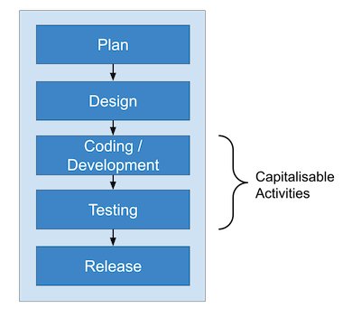
Costs can be capitalised once “technological feasibility” has been achieved. Topic 985 says that:
“the technological feasibility of a computer software product is established when the entity has completed all planning, designing, coding, and testing activities that are necessary to establish that the product can be produced to meet its design specifications including functions, features, and technical performance requirements.”
Agile doesn’t work that way. Agile does not have “one-and-done” stages of development since it is iterative; there is not necessarily a clear point at which “technological feasibility” is achieved; therefore the criteria for “technological feasibility” may be an important point to agree upon between client and vendor.
The problem is this: the guidelines state that the costs that should not be capitalized include the work that needs to be done to understand the product’s desired features and feasibility; these costs should be expensed as incurred costs.
For example, using development of external software (software developed for purchase or lease by external customers) as an example, the following activities cannot be capitalised:
- Upfront analysis
- Knowledge acquisition
- Initial project planning
- Prototyping
- Comparable design work
The above points apply even during iterations/sprints. If we wanted to be really pedantic, during development, the following activities cannot be capitalised either, but must be expensed:
- Troubleshooting
- Discovery
This may be an underlying reason why companies are leery of workshops and inceptions, because these probably end up as costs incurred instead of capitalised expenses. (Source)
Value Proposition: We should aim to optimise workshops and inceptions.
Capitalisable and Non-Capitalisable Costs for Cloud
For Cloud Costing, we have the following categories from an accounting perspective:
- Capitalizable Costs
- External direct costs of materials
- Third-party service fees to develop the software
- Costs to obtain software from third-parties
- Coding and testing fees directly related to software product
- Non-capitalisable Costs
- Costs for data conversion activities
- Costs for training activities
- Software maintenance costs
This link and Accounting for Cloud Development Costs are readable treatments of the subject. Also see this.
Articulating Value: The Value of a Software System
There is no consensus on how value of engineering practices should be articulated. Metrics like DORA metrics can quantify the speed at which features are released, but the ultimate consequences - savings in effort, eventual profits, for example – are seldom quantified. It is not that estimates of these numbers are not available; it is discussed when making a business case for the investment into a project, but those numbers are almost never encountered or leveraged by engineering terms to articulate how they are progressing towards their goal. The measure of progress across iterations is story points, which is useful, but that is just quantifying the run cost, instead of the actual final value that this investment will deliver.
How, then, do we then articulate this value?
Economics and current accounting practices can show one way forward.
One straightforward way to quantify software value is to turn to Financial Valuation techniques. Ultimately, the value of any asset is determined by the amount of money that the market wants to pay for it. Software is an intangible asset. Let’s take a simple example: suppose the company which owns/builds a piece of software is being acquired. This software could be for its internal use, e.g., accounting, order management, etc., or it could be a product that is sold or licensed to the company’s clients. This software needs to be valued as part of the acquisition valuation.
The question then becomes: how is the valuation of this software done?
There are several ways in which valuation firms estimate the value of software.
1. Cost Approach
This approach is usually used for valuing internal-use software. The cost approach, based on the principle of replacement, determines the value of software by considering the expected cost of replacing it with a similar one. There are two types of costs involved: reproduction costs and replacement costs. Reproduction Costs evaluate the cost of creating an exact copy of the software. Replacement Costs measure the cost of recreating the software’s functionality.
-
Trended Historical Cost Method: The trended historical cost method calculates the actual historical development costs, such as programmer personnel costs and associated expenses, such as payroll taxes, overhead, and profit. These costs are then adjusted for inflation to reflect the current valuation date. However, implementing this method can be challenging, as historical records of development costs may be missing or mixed with those of operations and maintenance.
-
Software engineering model method: This method uses specific metrics from the software system, like size/complexity, and feeds this information to some empirical software development models like COCOMO (Constructive Cost Model and its sequels) and SLIM (Software LIfecycle Management) to get estimated costs. The formulae in these models are derived from analyses of historical databases of actual software projects.
See Application of the Cost Approach to Value Internally Developed Computer Software: Williamette Management Associates for some comprehensive examples of this approach.
Obviously, this approach largely ignores the actual value that the software has brought to the organisation, whether it is in the form of reduced Operational Expenses, or otherwise.
2. Market Approach
The market approach values software by comparing it to similar packages and taking into account any variations. One issue with this method is the lack of comparable transactions, especially when dealing with internal-use software designed to specific standards. More data is available for transactions related to software development companies’ shares compared to software. This method could be potentially applicable to internal-use systems which are being developed even though there are commercial off the shelf solutions available; this could be because the COTS solutions are not exact fits to the problem at hand, or lack some specific features that the company could really do with.
3. Income Approach
The Income Approach values software based on its future earnings, or cost savings. The discounted cash flow method calculates the worth of software as the present value of its future net cash flows, taking into account expected revenues and expenses. The cash flows are estimated for the remaining life of the software, and a discount rate that considers general economic, product, and industry risks is calculated. If the software had to be licensed from a third party, its value is determined based on published license prices for similar software found in intellectual property databases and other sources.
The Income approach is usually the one used most often by corporate valuation companies when valuing intangible assets like software during acquisition. However, this software is usually assumed to be complete, and serving its purpose, and not necessarily software which is still in development (or not providing cash flows right now).
- Discounted cash flow method: This is the usual method where an NPV analysis is done on projected future cash flows arising from the product.
- Relief from Royalty Method: This method is used to determine the value of intangible assets by taking into account the hypothetical royalty payments that would be avoided by owning the asset instead of licensing it. The idea behind the RRM is straightforward: owning an intangible asset eliminates the need to pay for the right to use that asset. The RRM is commonly applied in the valuation of domain names, trademarks, licensed computer software, and ongoing research and development projects that can be associated with a particular revenue stream, and where market data on royalty and license fees from previous transactions is available. One possible example is if a company is building its own private cloud as an alternative to AWS; the value that the project provides could be calculated from the fees that are projected to be saved if the company did not use AWS for hosting its services.
Real Options Valuation
This is used when the asset (software) is not currently producing cash flows, but has the potential to generate cash flows in the future, incorporating the idea of the uncertain nature of these cash flows. The paper Modeling Choices in the Valuation of Real Options: Reflections on Existing Models and Some New Ideas discusses classic and recent advances in the valuation of real options. Specifically surveyed are:
- Black-Scholes Option Pricing formula: The original, rigid assumptions on underlying model, not originally intended for pricing real options
- Binomial Option Pricing Model: Discrete time approximation model of Black-Scholes; not originally intended for pricing real options
- Datar-Matthews Method: Simulation-based model with cash flows as expert inputs; no rigid assumptions around cash flow models
- Fuzzy Pay-off Method: Payoff treated as a fuzzy number with cash flows as expert input; no rigid assumptions
I admit that I’m partial to the Binomial Option Pricing Model, because the binomial lattice graphic is very explainable; we’ll cover the Binomial Option Pricing Model and the Datar-Matthews Method in a sequel.
What approach do we pick?
There is no one approach that can account for all types of software. At the same time, multiple approaches may be applicable to a single type of software, with varying degrees of importance. It is important to note that the following categories are not mutually exclusive. The map below shows the type of value analysis that could be done for each kind of investment or asset.
graph TD
platform[Platform] --> rov[Real Options Valuation]
external[Products with External Transactional Value] --> dcf[Discounted Cash Flow]
external --> market[Market]
internal[Internal-Use Products] --> opex_npv[OpEx NPV Analysis]
internal --> rrm[Relief from Royalty Method]
enterprise_modernisation[Enterprise Modernisation] --> rov
enterprise_modernisation --> opex_npv
maintenance[Maintenance] --> opex_npv
1. Platform
Use: Real Option Valuation
A platform by itself does not provide value; it is the opportunities that it creates to rapidly build and offer new products to the market that is its chief attraction. A platform also allows creating other types of options as well, like allowing the company to build customised products of the same type to enter into new markets. For example, a custom e-commerce platform not only creates options to higher volumes of sales transactions in the current country, but provides the options to deploy a custom e-commerce site in a new country.
2. Products providing External Transactional Value
Use: Income, Market
These cover software which enable e-commerce, or allow access to assets in exchange for money. In many situations, projected incoming cash flows are easier to predict because of historical data, and provide a direct link to the value of the software. It is to be noted that components of these product may be built on top of a platform themselves, so the platform itself might be valued using real option pricing, while these are the actual investments themselves.
Also, products like COTS e-commerce platforms are widely available, and thus can provide good benchmarks in terms of the value being provided by the custom implementation.
3. Internal-Use products
Use: OpEx NPV Analysis, Relief from Royalty, Market
These cover systems which are used to streamline operational processes inside the company, and thus reduce waste. It is to be noted that there might be second, third and n-th order effects of these systems, thus reasonable efforts should be made to articulate those effects to provide a lower bound on the value of these systems. In most cases (but maybe not all), these reductions apply to the operational expenses of the company, hence the NPV analysis of OpEx is suggested. Such systems may also have COTS alternatives, through subscription or outright purchase. In those cases, Relief from Royalty and Market methods are also valuable ways of benchmarking value.
4. Enterprise Modernisation initiatives
Use: Real Option Valuation, OpEx NPV Analysis
Enterprise Modernisation can have multiple objectives. It can target any combination of the following:
- Mitigation of risk (no one knows how the old code works, and long-time maintainers are retiring)
- Expansion of service capacity (to meet higher traffic)
- Decrease time to market for future features (it might take very long to add features to the current system)
Enterprise Modernisation can certainly benefit from an NPV analysis of Operational Expenses, but the main reason for undertaking modernisation is usually creating options for a more diverse product portfolio, or faster time to market for new features to continue retaining customers.
5. Maintenance
Use: OpEx NPV Analysis
Maintenance of production software which isn’t expected to evolve (much) is usually a matter of minimising production issues, and streamlining the operational pipeline which is already (hopefully) reliably delivering value. The primary metric for value in this case should be the expected reduction in operational expenses. If new features are added occasionally, positive cash flows may also figure in this NPV analysis.
Another approach to valuing software using different dimensions is discussed in the paper The Business Value of IT; A Conceptual Model for Selecting Valuation Methods. However, these are not methods that are strictly used by valuation firms. We’ve reproduced the selection model below.
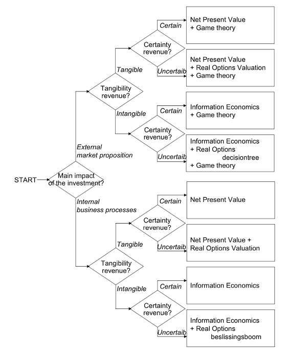
This paper also mentions using Information Economics to articulate value. Information Economics uses multiple criteria, both tangible and non-tangible, to come to a unified scorecard of value. Unfortunately, this does not have a monetary value attached to it for the intangible value creation processes. We may talk about it in the future. Information Economics: Managing IT Investment expounds upon this approach.
Articulating Value: The Cost of Reducing Uncertainty
We will use this spreadsheet again for our calculations. We spoke of the risk curve, which is the expected loss if the actual effort exceeds 310. Let us assume that the customer is adamant that we put in extra effort in narrowing our estimates so that we know whether we are over or below 310.
The question we’d like to answer is: how much are we willing to pay to reduce the uncertainty of this loss to zero? In other words, what is the maximum effort we are willing to spend to reduce the uncertainty of this estimate?
For this, we create a Loss Function, and this loss is simply calculated as \(L_i=P_i.E_i\) for every estimate \(i \geq 310\). Not too unsurprisingly, this is not the only choice for a loss function.
The answer is the area under the loss curve. This would usually done by integration, and is easily achieved if you are using a normal distribution, but is usually done through numerical integration for other arbitrary distributions. In this case, we can very roughly numerically integrate as shown in the diagram below, to get the maximum effort we are willing to invest.
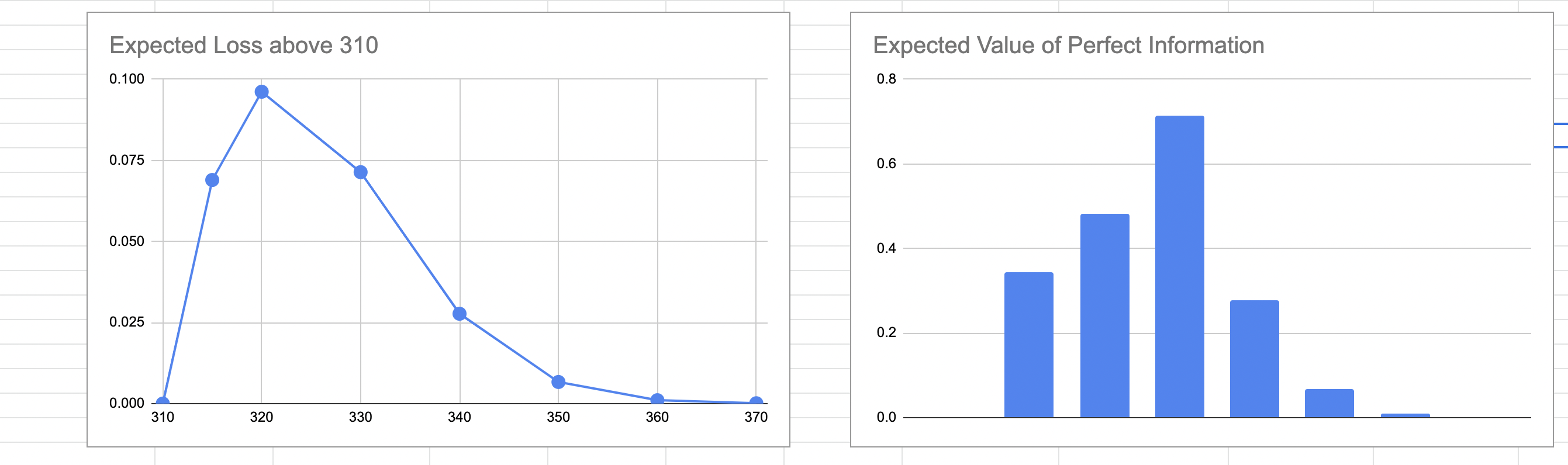
In our example, this comes out to 1.89. We can say that we are willing to make a maximum investment of 1.89 points of effort for the reduction in uncertainty to make economic sense. This value is termed the Expected Value of Information and is broadly defined as the amount someone is willing to pay for information that will reduce uncertainty about an estimate, or the information about a forecase. This technique is usually used to calculate the maximum amount of money you’d be willing to pay for a forecast about a business metric that affects your profits, but the same principle applies to estimates as well.
Usually, the actual effort to reduce the uncertainty takes far longer, and hopefully an example like this can convince you that refining estimates is not necessarily a productive exercise.
Articulating Value: The Cost of Expert but Imperfect Knowledge
Suppose you, the tech lead or architect, wants to make a decision around some architecture or tech stack. You’ve heard about it, and you think it would be a good fit for your current project scenario. But you are not completely sure, so in the worst case, there would be no benefit and just the cost sunk into the investment of implementing this decision. The two questions you’d like to ask are:
- What is the maximum I’m willing to pay to reduce the uncertainty of this decision completely? This question is exactly the same as the one in the previous section, so is not in itself that novel, but it is a stepping stone to the next question.
- What is the maximum I’m willing to pay to bring in an expert who can help me reduce this uncertainty to a lower value, but probably not to zero? In this case, the expert will not be able to provide you perfect information, and we must incorporate our confidence in the expert into our economics calculations.
We can use Decision Theory to quantify these costs. The technique we’ll be using involves Probabilistic Graphical Models, and all of this can be easily automated: this step-by-step example is for comprehension.
Suppose we have the situation above where a decision needs to be made. There is 30% possibility that the decision will result in a savings of $100000 going forward, and 70% possibility that there won’t be any benefit at all.
Let X be the event that there will be a savings of $20000. Then \(P(X)=0.3\). We can represent all the possibilities using a Decision Tree, like below.
graph LR
A ==>|Cost=5000| implement["Implement"]
A -->|Cost=0| dont_implement["Do Not Implement"]
implement ==>|"P(X)=0.3"| savings_1[Savings=20000-5000=15000]
implement ==>|"1-P(X)=0.7"| no_savings_1[Savings=0-5000=-5000]
dont_implement -->|"P(X)=0.3"| savings_2[Savings=0]
dont_implement -->|"1-P(X)=0.7"| no_savings_2[Savings=0]
Now, if we did not have any information beyond these probabilities, we’d pick the decision which maximises the expected payoff. The payoff from this decision is called the Expected Monetary Value, and is defined as:
\[EMV=\text{max}_i \sum_i P_i.R_{ij}\]This is simply the maximum expected value of all the expected values arising from all the choices \(j\in J\). The monetary value for the “Implement” decision is \(0.3 \times 15000 + 0.7 \times (-5000)=$1000\), whereas that of the “Do Not Implement” decision is zero. Thus, we pick the monetary value of the former, and our EMV is $1000.
Now assume we had a perfect expert who knew whether the decision is going to actually result in savings or not. If they told us the answer, we could effectively know whether to implement the decision or not with complete certainty.
The payoff then would be calculated using the following graph. The graph switches the chance nodes and the decision nodes, and for each chance node, picks the decision node which maximises the payoff.
graph LR
A ==> savings["Savings<br>P(X)=0.3"]
A ==> no_savings["No Savings<br>1-P(X)=0.7"]
savings ==>|Cost=5000| implement_1[Implement<br>Savings=20000-5000=15000]
savings -->|Cost=0| dont_implement_1[Don't Implement<br>Savings=0]
no_savings -->|Cost=5000| implement_2[Implement<br>Savings=0-5000=-5000]
no_savings ==>|Cost=0| dont_implement_2[Don't Implement<br>Savings=0]
We can then calculate expected payoff given perfect information (denoted as EV|PI) as:
\[EV|PI = \sum_i P_{j}.\text{max}_i R_{ij}\]In our case, this comes out to: \(0.3 \times 15000 + 0.7 \times 0=$4500\).
Thus the Expected Value of Perfect Information is defined as the additional amount we are willing to pay to get to EV|PI:
Thus, we are willing to pay a maximum of $3500 to fully resolve the uncertainty of whether our decision will yield the expected savings or not.
But the example we have described is not a real-world example. In the real world, even if we pay an expert to help us resolve this, they are not infallible. They might increase the odds in our favour, but there is always a possibility that they are wrong. We assume that we get an expert to consult for us. They want to be paid $3400. Are they overpriced or not?
We’d like to know what is the maximum we are willing to pay an expert if they can give us imperfect information about our situation. To do this, we will need to quantify our confidence in the expert.
Assume that if there are savings to be made, the expert says “Good” 80% of the time. If there are no savings to be made, the expert says “Bad” 90% of the time. This quantifies our confidence in the expert, and can be written as a table like so:
| Savings (S) / Expert (E) | Good | Bad |
|---|---|---|
| Savings | 0.8 | 0.1 |
| No Savings | 0.2 | 0.9 |
In the above table, E is the random variable representing the opinion of the expert, and S is the random variable representing the realisation of savings. We can again represent all possibilities via a probability tree, like so:
graph LR
A ==> savings["Savings<br>P(X)=0.3"]
A ==> no_savings["No Savings<br>1-P(X)=0.7"]
savings --> expert_good_1["Good<br>P(R)=0.8"]
savings --> expert_bad_1["Bad<br>1-P(R)=0.2"]
no_savings --> expert_good_2["Good<br>P(R)=0.1"]
no_savings --> expert_bad_2["Bad<br>1-P(R)=0.9"]
expert_good_1 --> p_1["P(Good,Savings)=0.3 x 0.8 = 0.24"]
expert_bad_1 --> p_2["P(Bad,Savings)=0.3 x 0.2 = 0.06"]
expert_good_2 --> p_3["P(Good,No Savings)=0.7 x 0.1 = 0.07"]
expert_bad_2 --> p_4["P(Bad,No Savings)=0.7 x 0.9 = 0.63"]
p_1-->p_good["P(Good)=0.24+0.07=0.31"]
p_3-->p_good
p_2-->p_bad["P(Bad)=0.06+0.63=0.69"]
p_4-->p_bad
We now have our joint probabilities \(P(S,E)\). What we really want to find is \(P(S \vert E)\). By Bayes’ Rule, we can write:
\[P(S|E)=\frac{P(S,E)}{P(E)}\]We can thus calculate the conditional probabilities of the payoff given the expert’s prediction with the following graph.
graph LR
p_1["P(Good,Savings)=0.3 x 0.8 = 0.24"]-->p_good["P(Good)=0.24+0.07=0.31"]
p_2["P(Bad,Savings)=0.3 x 0.2 = 0.06"]-->p_bad["P(Bad)=0.06+0.63=0.69"]
p_3["P(Good,No Savings)=0.7 x 0.1 = 0.07"]-->p_good
p_4["P(Bad,No Savings)=0.7 x 0.9 = 0.63"]-->p_bad
p_1 --> p_savings_good["P(Savings | Good)=0.24/0.31=0.774"]
p_good --> p_savings_good
p_2 --> p_savings_bad["P(Savings | Bad)=0.06/0.69=0.087"]
p_bad --> p_savings_bad
p_3 --> p_no_savings_good["P(No Savings | Good)=0.07/0.31=0.226"]
p_good --> p_no_savings_good
p_4 --> p_no_savings_bad["P(No Savings | Bad)=0.63/0.69=0.913"]
p_bad --> p_no_savings_bad
Now we go back and calculate EMV again in the light of these new probabilities. The difference in this new tree is that in addition to the probability branches of our original uncertainty, we also need to add the branches for the expert’s predictions, whose conditional probabilities we have just deduced.
graph LR
A ==>|0.31| p_good[Good]
A ==>|0.69| p_bad[Bad]
p_good ==> p_implement_good[Implement]
p_good --> p_dont_implement_good[Do Not Implement]
p_bad --> p_implement_bad[Implement]
p_bad ==> p_dont_implement_bad[Do Not Implement]

p_implement_good ==>|-5000| implement_savings_given_good["Savings=20000<br>P(Savings|Good)=0.774"]
p_implement_good ==>|-5000| implement_no_savings_given_good["Savings=0<br>P(No Savings|Good)=0.226"]
p_dont_implement_good -->|0| dont_implement_savings_given_good["Savings=0<br>P(Savings|Good)=0.774"]
p_dont_implement_good -->|0| dont_implement_no_savings_given_good["Savings=0<br>P(No Savings|Good)=0.226"]

p_implement_bad -->|-5000| implement_savings_given_bad["Savings=20000<br>P(Savings|Bad)=0.087"]
p_implement_bad -->|-5000| implement_no_savings_given_bad["Savings=0<br>P(No Savings|Bad)=0.913"]
p_dont_implement_bad ==>|0| dont_implement_savings_given_bad["Savings=0<br>P(Savings|Bad)=0.087"]
p_dont_implement_bad ==>|0| dont_implement_no_savings_given_bad["Savings=0<br>P(No Savings|Bad)=0.913"]

implement_savings_given_good ==> implement_savings_given_good_payoff["0.774 x (20000-5000)=11610"]
implement_no_savings_given_good ==> implement_no_savings_given_good_payoff["0.226 x (0-5000)=-1130"]
dont_implement_savings_given_good --> dont_implement_savings_given_good_payoff["0.774 x 0=0"]
dont_implement_no_savings_given_good --> dont_implement_no_savings_given_good_payoff["0.226 x 0=0"]

implement_savings_given_bad --> implement_savings_given_bad_payoff["0.087 x (20000-5000)=1305"]
implement_no_savings_given_bad --> implement_no_savings_given_bad_payoff["0.913 x (0-5000)=-4565"]
dont_implement_savings_given_bad ==> dont_implement_savings_given_bad_payoff["0.087 x 0=0"]
dont_implement_no_savings_given_bad ==> dont_implement_no_savings_given_bad_payoff["0.913 x 0=0"]

implement_savings_given_good_payoff ==> plus(("+"))
implement_no_savings_given_good_payoff ==> plus
plus ==> max_payoff_given_good[10480] ==> max_payoff[10480 X 0.31=3249]
Thus, $3249 is the maximum amount we’d be willing to pay this expert given the level of our confidence in them. This number is the Expected Value of Imperfect Information. Remember that the EVPI was $3500, so EVII <= EVPI. If you remember, the expert’s fee was $3400. This means that we would be overpaying the expert by $3400-$3249=$151.
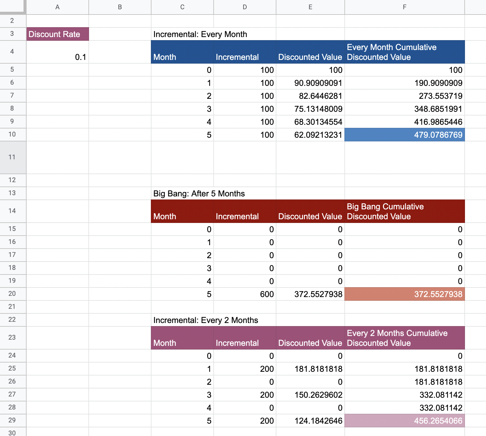
Articulating Value: The Cost of Unreleased Software
This spreadsheet contains all the calculations.
Static NPV Analysis Example: Circuit Breaker and Microservice Template
We show an example of articulating value for a simple (or not-sp-simple case), where multiple factors can be at play.
We are building a platform on Google Cloud Platform, consisting of a bunch of microservices. Many of these microservices are projected to call external APIs. Some of these APIs are prone to failure or extended downtimes; we need to be able to implement the circuit breaker pattern. We assume that one new microservice will be built per month for the next 6 months.
- The development cost of these microservices is $2000.
- The rate of return (hurdle rate) is 10%. This will be used to calculate the Net Present Value of future costs and benefits.
- These microservices also require ground-up work when creating a new one. A microservice template or starter pack would reduce work required to deploy future microservices as well.
Unfortunately, Istio is currently not being used. Istio is an open source service mesh that layers transparently onto existing distributed applications. If Istio was being used, we could have leveraged its circuit breaker pattern pretty easily. We need to advocate for using Istio in our ecosystem. Let us assume that currently we have no circuit breaker patterns implemented at all. How can we build a business case around this?
There are a couple of considerations:
- The deployment of the service mesh may be an expensive process.
- The microservice template could also encapsulate a library-level circuit breaker implementation.
- The microservice template would have other benefits that are not articulated in this example.
- Articulate Tech Debt due to No Circuit Breaker
- Articulate Library-level Circuit Breaker Option
- Articulate Microservice Starter Pack-level Circuit Breaker Option
- Articulate Service Mesh Circuit Breaker Option
- Explore combinations of these options
All the calculations are shown in this spreadsheet.
1. Articulate Tech Debt due to No Circuit Breaker
Suppose we analyse the downtime suffered by our platform per month because of requests piling up because of slow, or unresponsive third party APIs. We assume that this number is around $10000. This cost and that of new microservice development, are shown below.
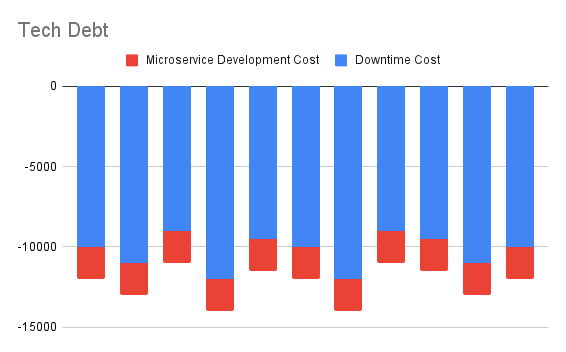
The current cash outflow projected over 10 months, discounted to today, comes out to -$87785. This is the first step towards convincing stakeholders that they are losing money. Of course, we can project further out into the future, but the uncertainty of calculations obviously grows the more you go out.
We’d like to propose a set of options
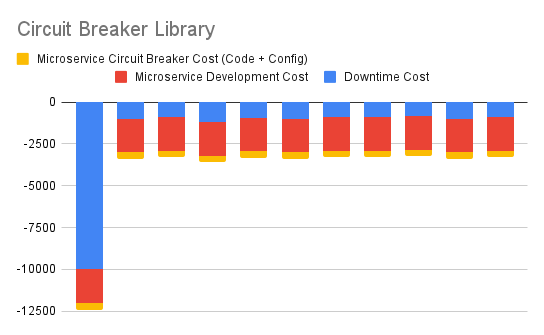
2. Articulate Immediate Library-level Circuit Breaker Option
This one shows cash flows arising out of immediately incorporating a circuit breaker library in each new microservice. The cost of incorporating this microservice includes any integration code as well as configuration. This effort remains more or less constant with each new microservice.
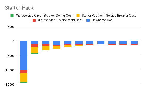
3. Articulate Immediate Starter Pack Option
This one shows cash flows arising out of immediately beginning to implement a Starter Pack which can be used as a template for building new microservices. Circuit breaker functionality is also included in this starter pack. Any integration code is also present in the pack by default. Note that the starter pack would normally also have other benefits, like preconfigured logging, error handling, etc.
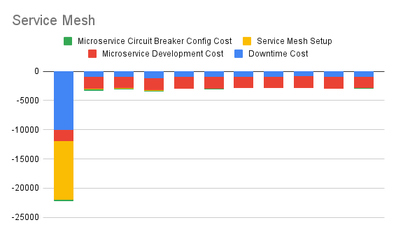
4. Articulate Immediate Service Mesh Option
This one shows cash flows arising out of immediately beginning to implement a Service Mesh.
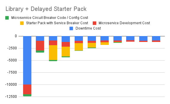
5. Articulate Immediate Library + Delayed Starter Pack Option
This option immediately starts integrating a circuit breaker library to reduce downtimes, but starts work on the starter pack a couple of months down the line. Once the starter pack is functional, explicit integration of the circuit breaker library will no longer be needed for each new microservice.
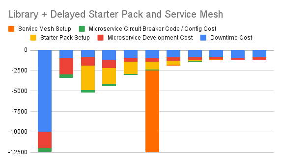
6. Articulate Immediate Library + Delayed Starter Pack Option + Delayed Service Mesh Option
This option is the same as above, except that later on, it also begins to implement a service mesh. Once the service mesh is complete, integration of the circuit breaker functionality in the starter pack will no longer be needed, but it will still continue to provide other benefits, like reducing initial setup time for a new microservice.
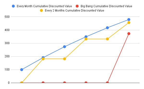
7. Review, Rank, and Choose
Here, we chart the (negative) discounted costs per month for all our options.
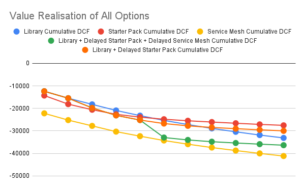
We may naively choose the one which has the least potential cost in the near horizon (which is the immediate starter pack option), or we can choose one of the service mesh options, assuming that service mesh is part of our architecture strategy, and that the cost differential is not too much. It is to be noted that for the service mesh to be part of our architecture strategy, other benefits of the service mesh need to be articulated using cash flows against the option of just having the starter pack do all those things.
Thus, it is not important to know which factors are being taken into account when doing the NPV analysis, and the final decision rests on all the relevant factors, not just an isolated one, like the one we presented in this example.
Conclusion
There are several other topics that we will defer to the next post. The following is a possible list of topics we’ll cover going forward.
- The Value of Security
- The Value of Pair Programming
- Value Chain Analysis
References
- Books
- Real Options Analysis
- Papers
- Real Options
- Valuation
- Illustrative Example of Intangible Asset Valuation: Shockwave Corporation
- The Valuation of Modern Software Investment in the US
- Information Technology Investment: In Search of The Closest Accurate Method
- The Business Value of IT; A Conceptual Model for Selecting Valuation Methods
- Software Economics: A Roadmap
- Web
- Information Economics
- Good Presentation on using multicriteria (tangible and non-tangible parameters) methods of Information Economics to link to software value
- Decision Theory
- Software Valuation
- Application of the Cost Approach to Value Internally Developed Computer Software: Williamette Management Associates
- Valuation of Software Intangible Assets by Willamette Management Associates
- Parameters of Software Valuation: Finantis Value
- Valuing Software Assets from an Accounting Perspective: EqVista
- Software Accounting
- Overview of Software Capitalisation Rules
- Accounting for external-use software development costs in an agile environment
- External Use Software guidelines - FASB Accounting Standards Codification (ASC) Topic 985, Software
- Internal Use Software guidelines - FASB Accounting Standards Codification (ASC) Topic 350, Intangibles — Goodwill and Other
- Accounting for internal-use software using Cloud Computing development costs
- Accounting for Cloud Development Costs are covered under FASB Subtopic ASC 350-40 (Customer’s Accounting for Implementation Costs Incurred in a Cloud Computing Arrangement That Is a Service Contact (ASC 350-40)).
- Financial Reporting Developments: Intangibles - goodwill and other. The actual formal document is here.
- Information Economics