Functional Analysis: Norms, Operators, and Some Theorems

Avishek Sen Gupta on 19 July 2021

This article expands the groundwork laid in Kernel Functions: Functional Analysis and Linear Algebra Preliminaries to discuss some more properties and proofs for some of the properties of functions that we will use in future discussions on Kernel Methods in Machine Learning, including (but not restricted to) the construction of Reproducing Kernel Hilbert Spaces.

However, in this article, we will expound more fundamentals concepts to build up our intuition. Thus, this (and some other articles) will serve as a “knowledge base” for applicable results in Real and Functional Analysis, and will be referenced in more future posts.

There is some more (unorganised) material in Functional and Real Analysis Notes which this post will also refer to.

We will discuss the following topics:

Metric Spaces and \(L^p\) Norms
Operators and Linear Functionals
\(L^p\) Norms
\(L^2\) and \(L^\infty\) Norms for Functions
Riesz Representation Theorem
Mercer’s Theorem

Operators and Linear Functionals

For the purposes of discussion, we may consider Operators as equivalent to Linear Transformations (there are nonlinear operators too, but that is outside the scope of this discussion). The term “operator” is used when these transformations are applied to a wide variety of inputs, usually beyond simple geometric notions of \(\mathbb{R}^n\).

In our discussions of applications of Functional Analysis, the most common application of operators will be on functions; but we may think of them as linear transformations under a different name. Note that they are still functions operating on vectors (because the inputs are functions, which are vectors themselves). For the results discussed in this article, we will restrict ourselves to Continuous Linear Operators.

Briefly then, an Operator is defined as \(T:X\rightarrow Y\), where \(X\) and \(Y\) are vector spaces.

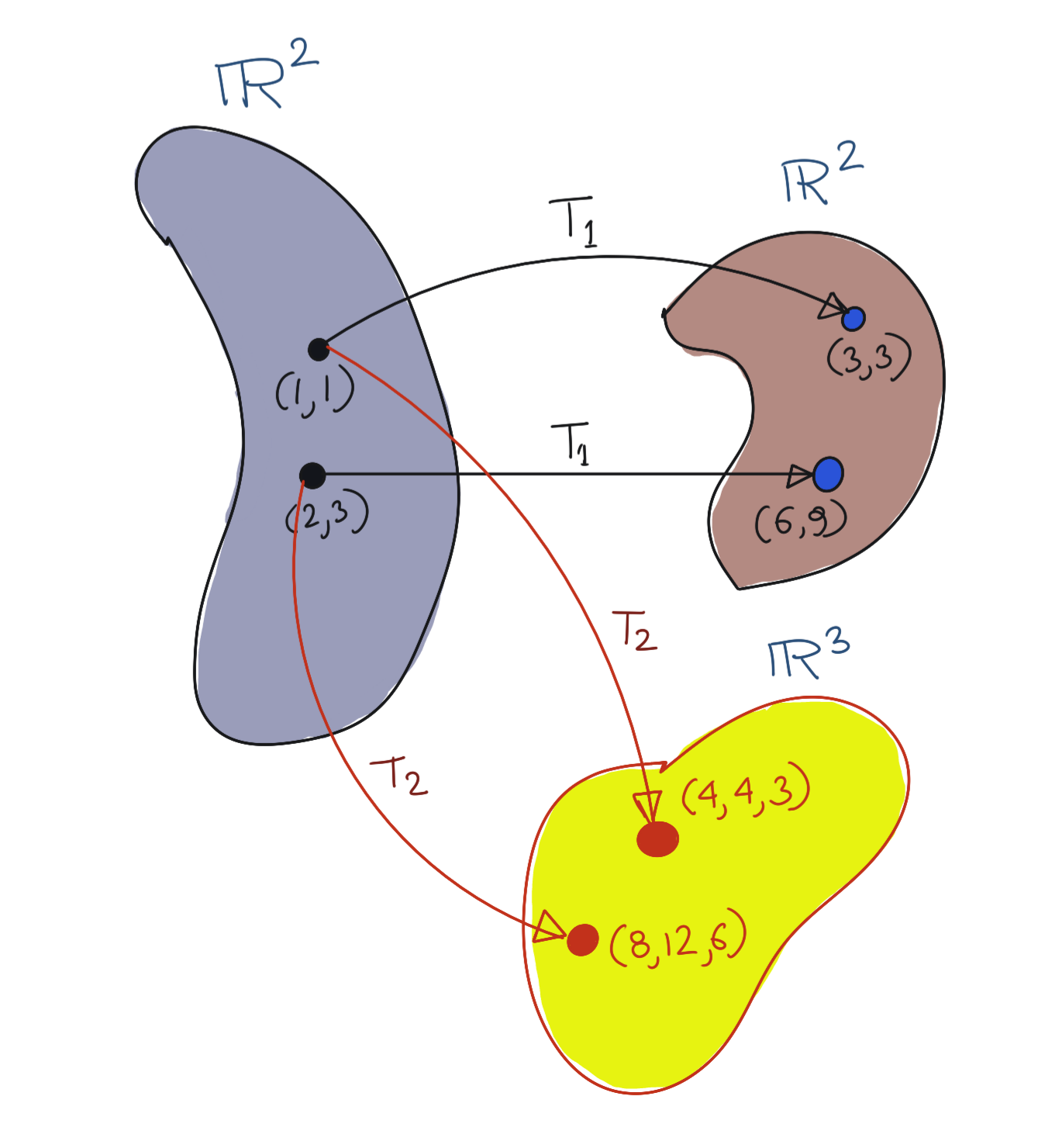Operator Examples Some examples of Operators, \(T_1:\mathbb{R}^2\rightarrow\mathbb{R}^2\) and \(T_2:\mathbb{R}^2\rightarrow\mathbb{R}^3\)

Linear Functionals are functions which map vectors specifically to their field of scalars, usually \(\mathbb{R}\) or \(\mathbb{C}\).

Briefly then, a Linear Functional is defined as \(f:X\rightarrow\mathbb{F}\), where \(X\) is a vector space. \(\mathbb{F}\) can be either \(\mathbb{R}\) (the real number line) or \(\mathbb{C}\) (the complex plane). For future discussions, we will simply use \(\mathbb{R}\).

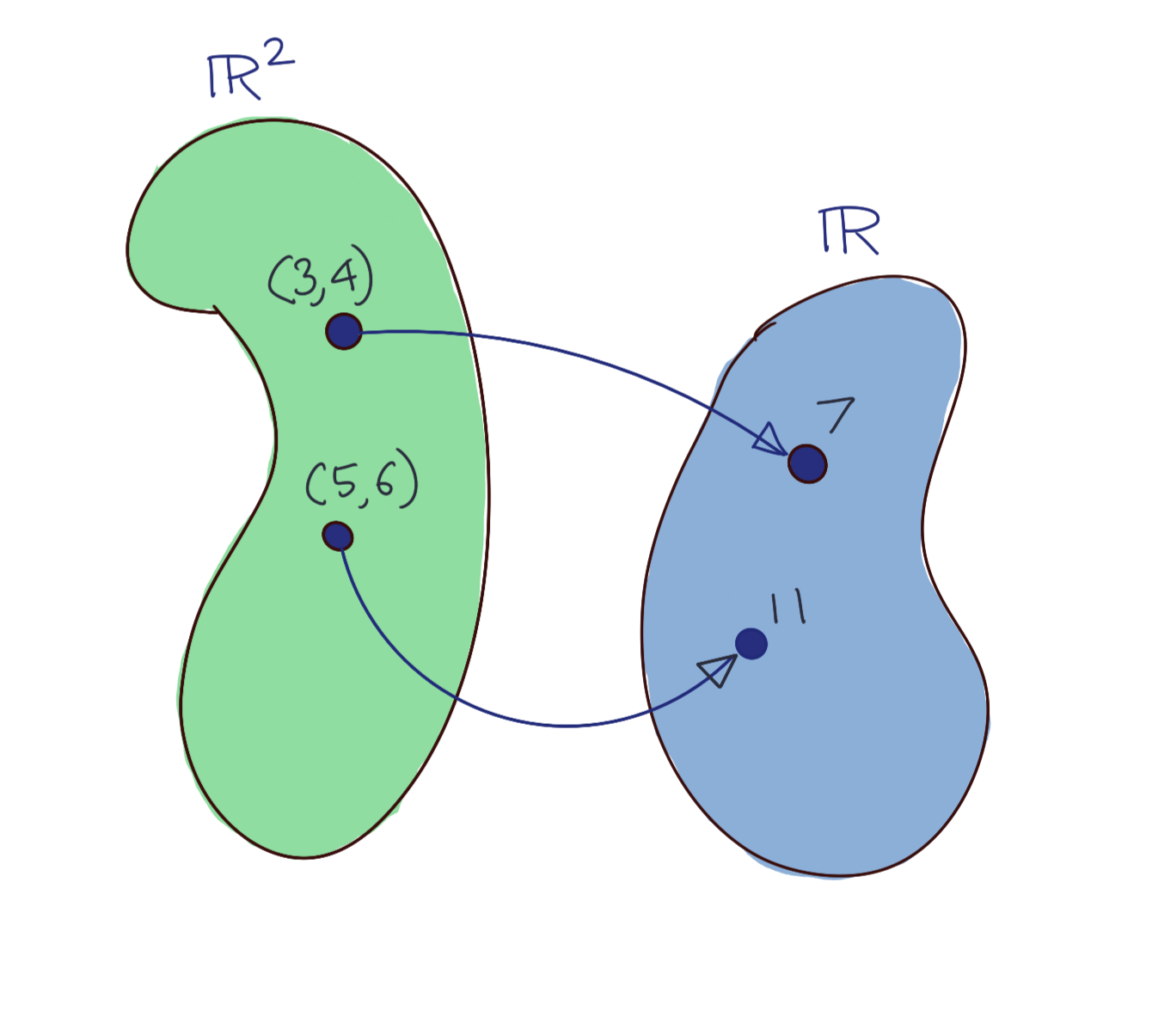Linear Functional Examples An example of a Linear Functional \(\mathbb{R}^2\rightarrow\mathbb{R}\)

By the way, Linear Functionals are also Operators because they are also linear transformations; it is just that they always map to a vector space over the field of scalars (specifically the field over which the linear functional was defined on).

Both Linear Functionals and Linear Operators obey two important rules:

\[L(\alpha x)=\alpha L(x)\]
\[L(x+y)=L(x)+L(y)\]

We will discuss the continuity aspect enjoyed by Continuous Linear Operators in an upcoming section.

We look at a couple of very simple examples of what does and does not constitute Linear Functionals.

Example of a Linear Functional

Let \(f(x)=2x, x\in\mathbb{R}\). Then, you can pick a constant \(C\), say \(C=3\), such that:

\[\|Tx\|=2\|x\|\leq 3\|x\|\]

Non-Example of a Linear Functional

As a non-example, consider \(f(x)=2x+3\). Note that this is not a linear transformation in \(R^n\); one intuitive reason is that there is no matrix you can define which can reproduce this operation when applied to any \(x\in\mathbb{R}\). This is despite the fact that this is a continuous function.

It is also not a Linear Functional because it does not follow one of the properties, as follows:

\[f(x_1+x_2)=2(x_1+x_2)+3=2x_1+2x_2+3 \\ f(x_1)+f(x_2)=2x_1+3+2x_2+3=2x_1+2x_2+6\\ \Rightarrow f(x_1+x_2)\neq f(x_1)+f(x_2)\]

Please note that this definition of linearity is not one that non-mathematicians are used to, since you’d normally look at an expression \(2x+3\) and conclude that it was “linear” in the sense that it expresses a polynomial of degree one, or alternatively, its graph is a straight line (or a plane in \(\mathbb{R}^3\), or an equivalent hyperplane in higher dimensions).

\(L^p\) Norms

Before discussing the norm of a function, let’s talk of the family of norms which include the natural concept of the Euclidean norm, namely the \(L^p\) norms.

The generalised \(L^p\) norm for a vector \(x\) in \(\mathbb{R}^n\) is defined as:

\[\|x\|_p={({\|x_1\|}^p + {\|x_2\|}^p + ... + {\|x_n\|}^p)}^{\frac{1}{p}} \\ \|x\|_p={(\sum_{i=1}^n {\|x_i\|}^p)}^{\frac{1}{p}}\]

The definition of the Euclidean distance metric falls out from the above definition immediately for \(p=2\). Interestingly, we see that other norms are possible. Say we put \(p=1\) above. Then we get the \(L^1\) norm defined as:

\[\|x\|_1=\|x_1\| + \|x_2\| + ... + \|x_n\|\]

Let us investigate the shapes traced by these norms to build a little geometric intuition, in \(\mathbb{R}^2\). To do this, we will trace the locii of points for which \(\|x\|_p=1\). That is, we will look at the locii for which the following norm equalities are satisfied.

\[\|x\|+\|y\|=1 \\ {({\|x\|}^2+{\|y\|}^2)}^{\frac{1}{2}}=1 \\ {({\|x\|}^3+{\|y\|}^3)}^{\frac{1}{3}}=1 \\ \vdots\]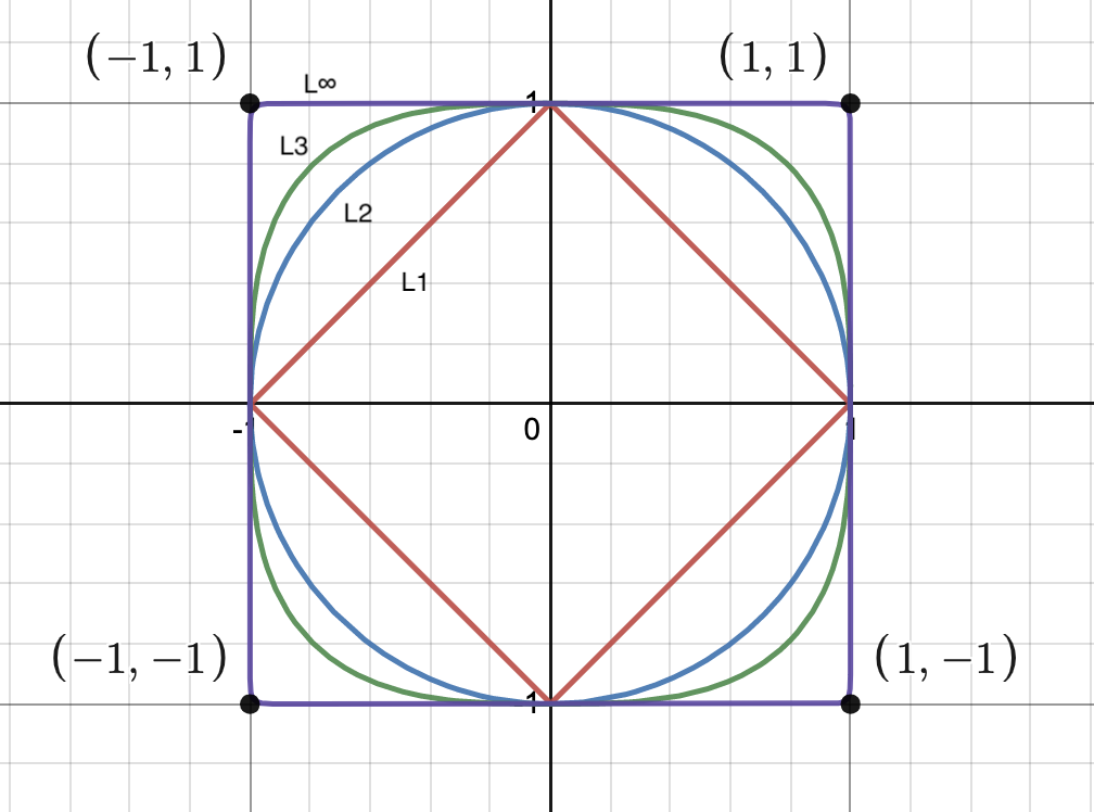

Lp Norms

As you can see, the \(L^2\) norm is the familiar unit circle given by \(x^2+y^2=1\). The other norms, however, look a little strange. However, this goes to show that the distance metric is a choice we actively make when building a metric space. Higher-powered \(L^p\) norms become “squarer” in shape.

The limiting case is the \(L^\infty\) norm which is essentially a square with corners at \((1,1)\), \((1,-1)\), \((-1,1)\), and \((-1,-1)\).

It can be proven that:

\[\|x\|_\infty=max(\|x_1\|, \|x_2\|, ..., \|x_n\|)\]

Intuitively, we can think of this definition like this: the magnitude of the largest vector component overpowers all other vector components, when it is raised to infinity.

Function Norms

With that discussion of norms, it should be clear now that different norms can be assigned to vector spaces of functions as well. The important point two remember is that functions have an infinite number of dimensions. Two of the common ones are as follows:

\(L^2\) Function Norm: The function is treated as a vector with an infinite number of dimensions similar to how we discussed in Kernel Functions: Functional Analysis and Linear Algebra Preliminaries. In this case, the function norm is identical to the norm induced by the Inner Product; though you should keep in mind that though the inner product induces this norm, this norm can be defined independently without the existence of an inner product in the space under discussion.

(An equivalent formulation exists: we can treat a function as an infinite sequence of scalars \(\{a_n\}=(a_1, a_2, a_3, ...)\). We will keep this treatment aside for now.)

The \(L^2\) function norm then looks like:
\[{\|f\|}_p=\int_a^b {\|f(x)\|}^2 dx\]
\(L^\infty\) Function Norm: This one boils down to simply finding out the maximum value attained by the function, or alternatively, the smallest value of \(C\in\mathbb{R}\) such that \(C>\|f(x)\|\) for all \(x\). The norm then becomes:
\[{\|f\|}_\infty={sup}_x\|f(x)\|\]
This is also referred to as the sup-norm of a function, and can be written as \({\|\|}_sup\).

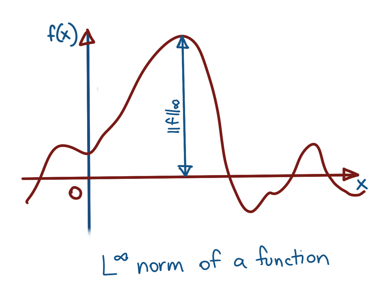Sup Norm of a Function

Operator Norm

The Operator Norm is not really a new way of describing a norm; it still depends upon the norms defined in vector spaces for the actual calculation. An operator norm is a measure of how much the operator modifies the norm of the original input vector.

Assume we have a vector \(x\) in a vector space \(X\), and an operator \(T:X\rightarrow Y\). Then its norm is \(\|x\|\). Applying the operator \(T\) on \(x\) gives us \(Tx\), whose norm in turn is \(\|Tx\|\). The degree of change in the norm is then given by \(\frac{\|Tx\|}{\|x\|}\). However, we want to find the maximum possible degree of change in norm, across all possible vectors in \(X\).

The operator norm is then defined as the maximum possible value of this ratio.

\[\|T\|={max}_{x}\frac{\|Tx\|_Y}{\|x\|_X}\]

The only problem with the above is that \(\|T\|\) will not be defined for \(x=0\). Thus, we conveniently exclude 0 from the definition, to give us the following:

\[\|T\|={max}_{x\neq 0}\frac{\|Tx\|_Y}{\|x\|_X}\]

Note the subscripts in the norms above. Since \(T\) takes \(x\) to a vector space \(Y\), the norm of \(x\) is measured using the norm defined in vector space \(X\), but the norm of \(Tx\) is measured using the norm defined in the vector space \(Y\).

There is a simpler way of expressing this: if we constrain \(x\) to always have a norm of 1, i.e., a unit vector, the denominator in the above expression becomes 1, so we can rewrite the operator norm as:

\[\|T\|={max}_{\|x\|=1}\|Tx\|_Y\]

I’ve omitted the norm subscript above, but remember that \(\|x\|=\|x\|_X\) in the above expression.

Metric Spaces

Sets don’t come naturally equipped with a way to measure “distances” between their elements. Some sets might have intuitive notions of what it means by distance between two elements in it, like n-dimensional Euclidean space (\(\mathbb{R}^n\)), but those intuitive metrics are not the only possible metrics available for those sets.

A set equipped with a distance metric is a metric space. A distance metric is defined as a function which defines the “distance” between two members of a set. The definition of what “distance” consititutes, varies based on the sort of metric space, and the application. A distance metric \(d(x,y)\) must satisfy the following conditions.

\[d(x,y)>0, \forall x\neq y\]
\[d(x,y)=0 \Rightarrow x=y\]
\[d(x,y)=d(y,x)\]
\[d(x,z)\leq d(x,y)+d(y,z)\]

Continuity of Functions

Continuity for a function can be defined as follows:

\[x\rightarrow x_0 \Rightarrow f(x)\rightarrow f(x_0)\\\]

Another equivalent definition for continuity is more useful:

\[d(x,x_0)\rightarrow 0\Rightarrow d(f(x), f(x_0))\rightarrow 0 \\\]

where \(d(\bullet, \bullet)\) is the distance metric defined for the metric space under discussion. However, the formulation that is used most commonly in proofs (in Real Analysis, etc.), is the \(\epsilon-\delta\) formulation. Mathematically, for a function \(f:X\rightarrow Y\), this is:

\[\forall \epsilon>0, \exists\delta>0 \text{ such that } d_X(x,x_0)<\delta \Rightarrow d_Y(f(x),f(x_0))<\epsilon \\ \forall \epsilon>0, \exists\delta>0 \text{ such that } \|x,x_0\|_X<\delta \Rightarrow {\|f(x) - f(x_0)\|}_Y<\epsilon \\\]

The two definitions above are equivalent, since a metric can be induced by a norm, and we will usually describe normed spaces. The \(d_X\), \(d_Y\), \(\|\bullet\|_X\), and \(\|\bullet\|_Y\) are there to make explicit the fact the norms (and by extension, the distance metric) might be different in the domain and the codomain.

Generally speaking, a mapping (a function is a mapping) is continuous if it preserves convergence in the codomain of the mapping. See Functional and Real Analysis Notes for more discussion on convergence.

Informally, this means that if there were two points \(x_1\), \(x_2\) in the domain \(X\) which were close to each other (closeness defined by the distance metric induced by the norm, or transitively, the inner product in \(X\): see Function Norms), then the corresponding mapped points \(f(x_1)\), \(f(x_2)\) in the codomain are also close to each other (closeness defined by some distance metric in the codomain).

Riesz Representation Theorem

Informally, the Riesz Representation Theorem states that every continuous (and therefore, bounded) linear functional \(f\) applied on a vector \(x\) in a vector space \(X\) is equivalent to the inner product of a unique vector (corresponding to \(f\)) with \(x\).

We’ll show a motivating example in finite-dimensional space \(\mathbb{R}^2\). Assume we have a vector \(\vec{z}=\begin{bmatrix}1\\2\end{bmatrix}\), and a function \(f(x)=2\vec{x}_1+3\vec{x}_2\).

Then there exists a vector \(\vec{v}=\begin{bmatrix}2\\3\end{bmatrix}\) corresponding to \(f\) such that \(f(\vec{z})=\langle\vec{v},\vec{z}\rangle\). Indeed, if we evaluate both sides, we get:

\[f(\vec{z})=2.1+3.2=8 \\ \langle\vec{v},\vec{z}\rangle=2.1+3.2=8\]

Mercer’s Theorem

Mercer’s Theorem is the functional (read infinite-dimensional) version of the eigendecomposition of a matrix. We present the equivalent forms without proof; we may tackle it in a more theoretical Functional Analysis post.

We talked about eigenvalues and eigenvectors briefly in Quadratic Optimisation using Principal Component Analysis as Motivation: Part Two, where we saw that symmetric matrices have orthogonal eigenvectors. There is also another property they enjoy in that all the eigenvalues are real-valued.

Symmetric Matrices and Orthogonal Eigenvectors

Here is a quick refresher proof on why symmetric matrices have orthogonal eigenvectors. Assume a symmetric matrix \(A=A^T\). Pick any two of its eigenvectors and corresponding eigenvalues, say \((\lambda_1, v_1)\) and \((\lambda_2, v_2)\), with the reasonable assumption that \(\lambda_1\neq\lambda_2\). Then we can write the following chain of identities:

\[\lambda_1{v_1}^Tv_2=(\lambda_1{v_1}^T)v_2={(Av_1)}^Tv_2={v_1}^TA^Tv_2 \\ = {v_1}^TAv_2 \text{ because A is symmetric} \\ = {v_1}^T(Av_2)={v_1}^T(\lambda_2v_2)=\lambda_2{v_1}^Tv_2 \\ \Rightarrow \lambda_1{v_1}^Tv_2 - \lambda_2{v_1}^Tv_2 = 0 \\ \Rightarrow (\lambda_1-\lambda_2){v_1}^Tv_2 = 0\]

Since we have assumed that \(\lambda_1\neq\lambda_2\), we get:

\[{v_1}^Tv_2 = 0\]

implying that all eigenvectors of a symmetric matrix are orthogonal to each other.

There will be a deeper delve into eigenvectors in a succeeding post.

Spectral Theorem for Finite-Dimensional Matrices

The infinite-dimensional version of an eigenvector is predictably called an eigenfunction. Let’s look at the finite-dimensional case to establish a direct visual equivalence with the statement of Mercer’s Theorem.

We take the case of a symmetric matrix which has strictly orthogonal real-valued eigenvectors, and then multiply out the matrices to see what \(A\) looks like.

Let

\[V= \begin{bmatrix} V_1 && V_2 && \ldots && V_n \\ \vert && \vert && \ldots && \vert \end{bmatrix} \\ \lambda= \begin{bmatrix} \lambda_1 && 0 && \ldots && 0 \\ 0 && \lambda_2 && \ldots && 0\\ \vdots && \vdots && \ddots && \vdots\\ 0 && 0 && \ldots && \lambda_n \end{bmatrix} \\\]

Then, expanding, we get:

\[A=V\lambda V^T =\begin{bmatrix} V_1 && V_2 && \ldots && V_n \\ \vert && \vert && \ldots && \vert \end{bmatrix} \cdot \begin{bmatrix} \lambda_1 && 0 && \ldots && 0 \\ 0 && \lambda_2 && \ldots && 0\\ \vdots && \vdots && \ddots && \vdots\\ 0 && 0 && \ldots && \lambda_n \end{bmatrix} \cdot \begin{bmatrix} V_1 && - \\ V_2 && - \\ \vdots \\ V_n && - \\ \end{bmatrix}\\ = \begin{bmatrix} \lambda_1 V_1 && \lambda_2 V_2 && \ldots && \lambda_n V_n \\ \vert && \vert && \ldots && \vert \end{bmatrix} \cdot \begin{bmatrix} V_1 && - \\ V_2 && - \\ \vdots \\ V_n && - \\ \end{bmatrix}\\ = \lambda_1 V_1{V_1}^T + \lambda_1 V_2{V_2}^T + \lambda_1 V_3{V_3}^T + ... + \lambda_1 V_n{V_n}^T \\ \Rightarrow A = \sum_{i=1}^n \lambda_i V_i{V_i}^T\]

The above is simply the statement of the Spectral Theory of Matrices.

Mercer’s Theorem: Spectral Theorem for Positive Semi-Definite Functions

Mercer’s Theorem is an extension of this to an infinite-dimensional matrix, where the eigenvectors are replaced by eigenfunctions (remember, functions are vectors too), and the requirement for a symmetric matrix is replaced by a positive semi-definite function \(\kappa(x,y)\), characterised by the positive semi-definiteness of the Gram Matrix as noted in the Inner Product and the Gram Matrix section in Kernel Functions: Functional Analysis and Linear Algebra Preliminaries.

Mathematically, Mercer’s Theorem states that:

\[\kappa(x,y)=\sum_{i=1}^\infty \lambda_i \psi_i(x)\psi_i(y)\]

where \(\kappa(x,y)\) is a positive semi-definite function and \(\psi_i(\bullet)\) is the \(i\)th eigenfunction. Note that this implies that there are an infinite number of eigenfunctions.

References

tags: Mathematics - Theory - Operator Theory - Functional Analysis - Pure Mathematics

Total Internal Reflection

Code

Contact