Kernel Functions with Reproducing Kernel Hilbert Spaces

Avishek Sen Gupta on 20 July 2021

---

This article uses the previous mathematical groundwork to discuss the construction of Reproducing Kernel Hilbert Spaces. We’ll make several assumptions that have been proved and discussed in those articles. There are multiple ways of discussing Kernel Functions, like the Moore–Aronszajn Theorem and Mercer’s Theorem. We may discuss some of those approaches in the future, but here we will focus on the constructive approach here to characterise Kernel Functions.

The specific posts discussing the background are:

• Kernel Functions: Functional Analysis and Linear Algebra Preliminaries
• Functional Analysis: Norms, Linear Functionals, and Operators
• Functional and Real Analysis Notes

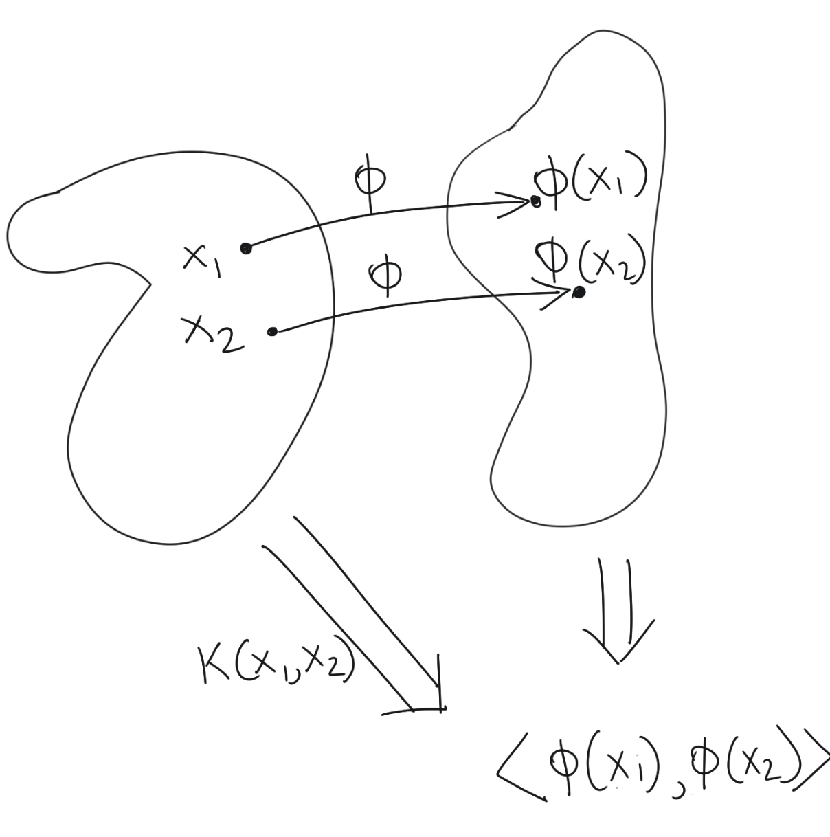
We originally asked the following question: what can we say about a function on a pair of input vectors which also ends up being the inner product of those vectors projected onto a higher dimensional space?

If we can answer this question, then we can circumvent the process of projecting a pair of vectors into higher-dimensional space, and then computing their inner products; we can simply apply a single function which gives us the inner products in higher dimensional space.

Proof by Construction

Mathematically, we are looking for a few things:

• A mapping function \(\phi(x)\): The mapping function projects our input into a higher-dimensional space.
• A definition of an inner product operation \(\langle\bullet, \bullet\rangle\): We already know (or think we know) that this inner product is the same as our intuitive understanding of an inner product, but we’ll see.
• A kernel function \(\kappa(x,y)\) which performs both of the above operations in one shot, i.e., \(\kappa(x,y)=\langle\Phi(x)\cdot\Phi(y)\rangle\).

There are three properties that a valid inner product operation must satisfy: we discussed them in Kernel Functions: Functional Analysis and Linear Algebra Preliminaries. This implies that \(\kappa\) must satisfy these properties. I reproduce them below for reference.

• Positive Definite: \(\kappa(x,x)>0\) if \(x\neq 0\)
• Principle of Indiscernibles: \(x=0\) if \(\kappa(x,y)=0\)
• Symmetric: \(\kappa(x,y)=\kappa(y,x)\)
• Linear:
  • \[\kappa(\alpha x,y)=\alpha\kappa(x,y), \alpha\in\mathbb{R}\]
  • \[\kappa(x+y,z)=\kappa(x,z)+\kappa(y,z)\]

We will alter our original question slightly to give some motivation for this proof. We ask the following:

• Is there a Hilbert space where the kernel function \(\kappa\) we choose is a valid inner product operation?
• If so, what does the projecting function \(\Phi\) look like?

Now, recall the criterion for positive semi-definiteness for a Gram matrix of \(n\) data points. Translated into polynomial form, it looked like this:

\[\begin{equation} \sum_{j=1}^n\sum_{i=1}^n\alpha_i\alpha_j\kappa(x_j, x_i) \geq 0 \label{eq:psd_criterion} \end{equation}\]

You can see immediately, that for \(n=1\), and \(\alpha_1=1\), the above simplifies to \(\kappa(x_1,y_1)=\kappa(x,y)\geq 0\). This immediately gives us a hint about functions for which positive semi-definite matrices can be constructed out of all data points (without making any assumptions about those data points); they are good candidates for kernel functions. Note that the above simplification results from having a single data point in our data set.

Furthermore, if \(\kappa\) is symmetric, the Gram matrix will be symmetric because \(G_{ij}=\kappa(x_i, x_j)=\kappa(x_j, x_i)=G_{ji}\).

So there is definitely strong evidence of positive semi-definite functions being kernel functions, but we need to add a little more rigour to our intuition. For example, we still have no idea what the mapping function \(\Phi\) should look like.

Linear Combinations of Positive Semi-Definite Matrices

There are two more points from the above exploratory analysis that is worth discussing, because we will be using it in our proof.

• The sum of positive semi-definite matrices is also positive semi-definite. Take two positive semi-definite matrices \(A\) and \(B\). Then, by definition of positive semi-definiteness, \(v^TAv\geq 0\) and \(v^TBv\geq 0\). So if we write:

  \[v^T(A+B)v=(v^TA+v^TB)v=\underbrace{\underbrace{v^TAv}_{\geq 0}+\underbrace{v^TBv}_{\geq 0}}_{\geq 0}\]

• Positive semi-definite matrices scaled by non-negative scalars \(\alpha\geq 0, \alpha\in\mathbb{R}\) are also positive semi-definite. This is because:

  \[v^T(\underbrace{\alpha}_{\geq 0} A)v= \underbrace{\underbrace{\alpha}_{\geq 0}\underbrace{v^TAv}_{\geq 0}}_{\geq 0}\]

The practical implication, as we will see, is that non-negative linear combinations of kernel functions are also kernel functions. In practice, the proof will use a set of kernel functions defined by a particular set of data points as basis vectors and use those to define a vector space of kernel functions. Any function in this space will then necessarily be a kernel function as well because of the implications we just discussed.

Exploring the Kernel

We will proceed to the general case of infinite-dimensional kernels by means of a simpler finite-dimensional motivating example. Assume that we already know the mapping \(\phi(x)\)of the input space (\(\mathbb{R}^2\)) to the feature space (\(\mathbb{R}^3\)), that is:

\[\phi:\mathbb{R}^2\rightarrow\mathbb{R}^3 \\ \phi(x)=\begin{bmatrix}x_1 \\ x_2 \\ x_1x_2\end{bmatrix}\]

Then we know what our kernel \(\kappa(x,y)\) should look like.

\[\kappa(x,y)=\langle\phi(x),\phi(y)\rangle ={\phi(x)}^T\phi(y) \\ = \begin{bmatrix}x_1 && x_2 && x_1x_2\end{bmatrix} \begin{bmatrix}y_1 \\ y_2 \\ y_1y_2\end{bmatrix}\]

Let us assume that a vector \(X\in\mathbb{R}^2\) has already been lifted to \(\mathbb{R}^3\), using \(\phi\). Then the mapped vector is \(\phi(X)\). Now, we pick an arbitrary linear functional \(f\) (it will turn out to be not so arbitrary later on) which acts on \(\phi(X)\) to give us some scalar in \(\mathbb{R}\).

The Riesz Representation Theorem states that for every (continuous) linear functional, there is a unique vector which does the same job when the inner product is computed between it and the input vector. This implies that there is a unique vector \(f_v\) which corresponds to \(f\), which can be used as part of the inner product, to do the same thing that \(f\) was doing.

To make it more concrete, suppose \(f(x)=x_1+x_2+x_1x_2\). Then the vector \(f_v=\begin{bmatrix}1 \\ 1 \\ 1\end{bmatrix}\).

Thus, we can write the following:

\[f(\phi(X))=\langle f_v, \phi(X)\rangle \\ ={f_v}^T\phi(X) \\ = \begin{bmatrix}1 && 1 && 1\end{bmatrix} \begin{bmatrix}X_1 \\ X_2 \\ X_1X_2\end{bmatrix} \\ = X_1+X_2+X_1X_2\]

This is where we need to shift our perspective. Because the inner product is symmetric (we will show this later), we can write:

\[f(\phi(X))=\langle f_v, \phi(X)\rangle \\ =\langle \phi(X), f_v\rangle=\phi_X(f_v)\]

This is like a reverse application of the Riesz Representation Theorem: instead of a function \(f\) acting on a vector \(\phi(X)\), we can think of a function \(\phi_X\) acting on a vector \(f_v\).

This implies that \(\phi_X\) is of the form:

\[\begin{equation} \phi_X(z)= \begin{bmatrix}X_1 && X_2 && X_1X_2\end{bmatrix} \begin{bmatrix}z_1 \\ z_2 \\ z_3\end{bmatrix} \label{eq:partial_feature_map} \end{equation}\]

Let us now curry the kernel function by specifying \(x=X\), so that we get:

\[\begin{equation} \kappa(X,\bullet)=\begin{bmatrix}X_1 && X_2 && X_1X_2\end{bmatrix} \begin{bmatrix}y_1 \\ y_2 \\ y_1y_2\end{bmatrix} \label{eq:partial_kernel} \end{equation}\]

There is a very close correspondence between the two forms \(\eqref{eq:partial_feature_map}\) and \(\eqref{eq:partial_kernel}\). This suggests that as long as the form of the function \(f\) “looks like \(\phi(x)\)“ (or is a scaled version; also remember that \(z\) started out as a linear functional \(f\)), we can set:

\[\phi_X(\bullet)=\kappa(X,\bullet)\]

because then for any \(\phi\)-like input to \(\phi_X(\bullet)\), we’d get:

\[\phi_X(Y)= \begin{bmatrix}X_1 && X_2 && X_1X_2\end{bmatrix} \begin{bmatrix}Y_1 \\ Y_2 \\ Y_1Y_2\end{bmatrix}\\ =\langle\phi(X),\phi(Y)\rangle\]

Using the same argument for a different vector \(Y\), we can then summarise both \(\phi(X)\) and \(\phi(Y)\):

\[\begin{equation} \phi_X(\bullet)=\kappa(X,\bullet) \label{eq:x_partial_kernel} \end{equation}\] \[\begin{equation} \phi_Y(\bullet)=\kappa(Y,\bullet) \label{eq:y_partial_kernel} \end{equation}\]

Now, we know that the vector dual (appealing to the Riesz Representation Theorem again) of \(\phi_X(\bullet)\) is \(\begin{bmatrix}X_1 \\ X_2 \\ X_1X_2\end{bmatrix}\). The vector dual of \(\phi_Y(\bullet)\) is \(\begin{bmatrix}Y_1 \\ Y_2 \\ Y_1Y_2\end{bmatrix}\). This implies that these functions are simply vectors.

Then, their inner product looks like so:

\[\langle\phi_X(\bullet), \phi_X(\bullet)\rangle=\begin{bmatrix}X_1 && X_2 && X_1X_2\end{bmatrix} \begin{bmatrix}Y_1 \\ Y_2 \\ Y_1Y_2\end{bmatrix}\\ = \kappa(X,Y)\]

Then by the above identities \(\eqref{eq:x_partial_kernel}\) and \(\eqref{eq:y_partial_kernel}\), we conclude that:

\[\mathbf{\kappa(x,y)=\langle\kappa(x,\bullet)\kappa(y,\bullet)\rangle}\]

This is the Reproducing Kernel Property, and it is the property which gives Reproducing Kernel Hilbert Spaces their name.

Verification of Inner Product properties

There is still some more bookkeeping to be done: we need to verify that the inner product we have defined, satisfies all the properties of an Inner Product, which are listed here.

Remember how we talked in Function Forms about any function we apply to on the projected point \(\phi(X)\) needs to “look like \(\phi(x)\)”? That essentially implies that this function needs to be a linear combination of a bunch of \(\phi(X_i)\)’s.

Each \(X_i\) in the original data set creates a new \(\phi_{X_i}\), and these function can be a linear combination of these. This implies that any such valid function looks like:

\[f(\bullet)=\sum_{i=1}^n\alpha_i \phi_{X_i}(\bullet) \\ =f(\bullet)=\sum_{i=1}^n\alpha_i \kappa({X_i},\bullet)\]

For clarity, we will continue to use the bullet notation.

Let’s take two such functions. We have already defined \(f\), so the other one is:

\[g(\bullet)=\sum_{j=1}^m\beta_i \kappa({X_j},\bullet)\]

We can choose a different set of basis functions for \(f\) and \(g\); hence it is possible that \(m\neq n\). Now, we take the inner product of \(f\) and \(g\):

\[\langle f(\bullet),g(\bullet)\rangle=\sum_{i=1}^n \sum_{j=1}^m \alpha_i\beta_j \kappa(X_i,\bullet) \kappa(X_j,\bullet) \\ =\sum_{j=1}^m \beta_j f(X_j) \\ =\sum_{i=1}^n \alpha_i g(X_i)\]

The above identities imply that the inner product is symmetric and linear.

We’d like to prove that the inner product is also positive definite. Recall that our kernel function is positive semi-definite if \(\eqref{eq:psd_criterion}\) is satisfied, that is:

\[\sum_{j=1}^n\sum_{i=1}^n\alpha_i\alpha_j\kappa(x_j, x_i) \geq 0\]

Since we have assumed that we are working with a positive semi-definite kernel, the inner product is proven to be positive semi-definite, at least. If \(\langle f,f\rangle=0\), then we can easily see that \(f=0\), thus the inner product is also positive definite, and the Principle of Indiscernibles is also satisfied.

Extension to Infinite Dimensions

The above motivating example was a finite dimensional case. Does this work in infinite dimensions, in cases where you cannot enumerate a vector completely, because it is a function with infinite dimensions? Yes, it does. The line of thinking continues to stay the same, though the kernel functions assume more complicated expressions than simple matrix products.

Addendum: Function Currying

Partial evaluation of a kernel function \(\kappa(x,y)\) is closely related to the notion of function currying from programming, where specifying a subset of arguments to a function, yields a new function with the already-passed-in parameters fixed, and the rest of the parameters still available to specify.

If we specify one of the parameters of \(\kappa(x,y)\), say \(y=Y\), this yields a new function with \(y\) fixed to \(Y\) and \(x\) still available to specify. We use the common notation used for common functions, by putting a dot in the place of the unspecified variables. We write it like so:

\[\kappa(x,y)=\kappa(\bullet,\mathbf{Y})\]

---