Non-Linear Support Vector Machines: Radial Basis Function Kernel and the Kernel Trick

Avishek Sen Gupta on 7 August 2021

---

This article builds upon the previous material on kernels and Support Vector Machines to introduce some simple examples of Reproducing Kernels, including a simplified version of the frequently-used Radial Basis Function kernel. Beyond that, we finally look at the actual application of kernels and the so-called Kernel Trick to avoid expensive computation of projections of data points into higher-dimensional space, when working with Support Vector Machines.

The specific posts discussing the background are:

• Support Vector Machines from First Principles: Part One
• Support Vector Machines from First Principles: Linear SVMs
• Kernel Functions: Kernel Functions with Reproducing Kernel Hilbert Spaces
• Kernel Functions: Functional Analysis and Linear Algebra Preliminaries
• Functional Analysis: Norms, Linear Functionals, and Operators
• Functional and Real Analysis Notes

We will discuss the following:

• Polynomial Kernels
• A simplified version of the popular Radial Basis Function kernel
• Non-Linear Support Vector Machines and the Kernel Trick

Even though we will look at specific feature maps for selected kernel functions in the next section, please note that feature maps induced by kernel functions are not unique. More than one feature map may exist for a given kernel function. Kernel functions only guarantee that we project our data into some higher-dimensional space; we do not always know (or care about) the actual feature space our data is being projected onto, only that it is.

Polynomial Kernels

Polynomial kernels are probably the simplest to understand; they are not necessarily used in practice (except for Natural Language Processing, source: Wikipedia), but are a good stepping-stone to understanding the infinite-dimensional scenarios.

Homogenous Polynomial Kernels (No Constant Term)

We start with an example of a simplified form of the polynomial kernel, without constants. These are called Homogenous Kernels.

This example is specific for vectors in \(\mathbb{R}^2\); we will be lifting them to \(\mathbb{R}^3\). The kernel function is \(\kappa(x,y)={\langle x,y\rangle}^2\). Incidentally, the kernel function will work with any \(\mathbb{R}^n\) domain of vectors, but for illustration purposes, we will stick to \(\mathbb{R}^2\).

Assume the vectors are \(X=\begin{bmatrix}X_1 \\ X_2\end{bmatrix}\) and \(Y=\begin{bmatrix}Y_1 \\ Y_2\end{bmatrix}\), and the inner product is the usual inner product defined in Euclidean space, i.e., \(\langle x,y\rangle=x^Ty\).

\[\kappa(x,y)={\langle x,y\rangle}^2\\ ={(X_1Y_1+X_2Y_2)}^2={(X_1Y_1)}^2+{(X_2Y_2)}^2+2X_1Y_1X_2Y_2\]

We’d like to know what mapping function \(\phi(x)\) (or equivalently, \(\kappa(x, \bullet)\)) projects our original points \(X\) and \(Y\) to \(\mathbb{R}^3\), so that the inner product in this new vector space is equal to the evaluation of the kernel function \(\kappa(x,y)\).

Because I know the answer already, we will write it straight away.

\[\phi(x)=\kappa(x,\bullet)=\begin{bmatrix}{x_1}^2 \\ {x_2}^2 \\ \sqrt 2x_1x_2 \end{bmatrix}\]

You can verify yourself that this satisfies the requirement of \(\kappa(x,y)=\langle\phi(x)\phi(y)\rangle\).

\[\langle\phi(x)\phi(y)\rangle=\begin{bmatrix}{X_1}^2 && {X_2}^2 && \sqrt 2X_1X_2 \end{bmatrix}\cdot \begin{bmatrix}{Y_1}^2 \\ {Y_2}^2 \\ \sqrt 2Y_1Y_2 \end{bmatrix}\\ = {(X_1Y_1+X_2Y_2)}^2={(X_1Y_1)}^2+{(X_2Y_2)}^2+2X_1Y_1X_2Y_2 \\ ={\langle x,y\rangle}^2=\kappa(x,y)\]

General Polynomial Kernel

The kernel function described above is a special case of the General Polynomial Kernel, which is of the form (again assuming the Euclidean version of inner product \(x^Ty\)):

\[\kappa(x,y)={(x^Ty+c)}^d\]

where \(c\in\mathbb{R}\) and \(d\in\mathbb{N}\) to. Note that \(d\) does not represent the number of dimensions that the vector will be lifted to.

Let’s look at a slight generalisation for a vector \(\mathbb{R}^n\) for \(d=2\), using the application of the Binomial Theorem.

\[\kappa(x,y)={(x^Ty+c)}^2={\left(\sum_{i=1}^nx_iy_i+c\right)}^2 \\ = {\left(\sum_{i=1}^nx_iy_i\right)}^2 + 2c\left(\sum_{i=1}^nx_iy_i\right) + c^2 \\ = \sum_{i=1}^n{(x_iy_i)}^2 + 2\sum_{i=1}^{n-1}\sum_{j+1}^n (x_ix_j)(y_iy_j) + 2c\left(\sum_{i=1}^nx_iy_i\right) + c^2 \\ = \sum_{i=1}^n{(x_iy_i)}^2 + \sum_{i=1}^{n-1}\sum_{j+1}^n (\sqrt{2}x_ix_j)(\sqrt{2}y_iy_j) + \left(\sum_{i=1}^n\sqrt{2c}x_i\sqrt{2c}y_i\right) + c^2 \\\]

Through visual inspection (or by expanding the above and noting the pattern of the polynomial), we can infer the mapping \(\phi\) as;

\[\phi(x)=\begin{bmatrix} {x_1}^2 \\ {x_1}^2 \\ \vdots \\ {x_n}^2 \\ \sqrt{2}x_1x_2 \\ \sqrt{2}x_1x_3 \\ \vdots \\ \sqrt{2}x_1x_n \\ \sqrt{2}x_2x_3 \\ \sqrt{2}x_2x_4 \\ \vdots \\ \sqrt{2}x_2x_n \\ \vdots \\ \sqrt{2}x_{n-1}x_n \\ \sqrt{2c}x_1 \\ \sqrt{2c}x_2 \\ \vdots \\ \sqrt{2c}x_n \\ c \end{bmatrix}\]

Similar mappings for higher values of \(d\) can be inferred by applying the Multinomial Theorem.

Radial Basis Function Kernel

The Radial Basis Function Kernel the most common kernel used in Machine Learning applications. The kernel function is of the form of a Gaussian function (Normal distribution). The simplest one-dimensional Gaussian is given by:

\[f(x)=C\cdot exp\left( -\frac{ {(x-\mu)}^2}{2\sigma_K^2}\right)\]

The forms of the kernel function for the one-dimensional, and the more general case (where a norm is induced by an inner product), are shown below.

\[\kappa(x,y)=C\cdot exp\left(- \frac{ {(x-y)}^2}{2\sigma_K^2}\right) \\ \kappa(x,y)=C\cdot exp\left(- \frac{ {\|x-y\|}^2}{2\sigma_K^2}\right)\]

We will prove that \(\kappa(x,y)\) is a Reproducing Kernel for the simple one-dimensional case. We will want to prove:

\[\kappa(x,y)=\langle\phi(x)\phi(y)\rangle\]

If we denote the free parameter as \(\mu\), we can write the following:

\[\phi_x(\mu)=a\cdot exp\left(- \frac{ {(x-\mu)}^2}{2\sigma^2}\right) \\ \phi_y(\mu)=a\cdot exp\left(- \frac{ {(y-\mu)}^2}{2\sigma^2}\right)\]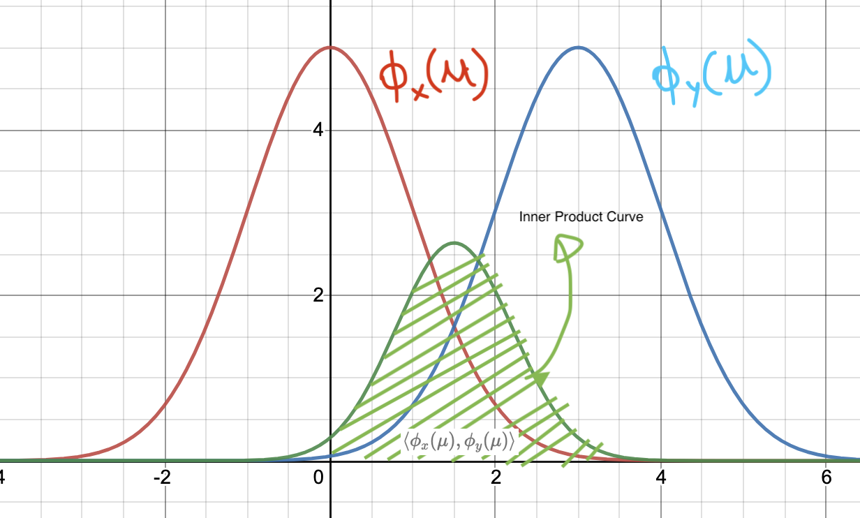

Inner Product Curve of two Gaussian Feature Maps

We need take the inner product of the above functions. Remember from Kernel Functions: Functional Analysis and Linear Algebra Preliminaries that the taking the inner product of two function amounts to taking the integral of their products, like so:

\[{\langle f,g\rangle}=\int_a^b f(x)g(x)dx\]

In this case, the limits are \((-\infty,+\infty)\), so we write:

\[{\langle \phi_x(\mu),\phi_y(\mu)\rangle}=\int_{-\infty}^{+\infty} a\cdot exp\left(- \frac{ {(x-\mu)}^2}{2\sigma^2}\right)\cdot a\cdot exp\left( -\frac{ {(y-\mu)}^2}{2\sigma^2}\right)d\mu \\ =a^2 \int_{-\infty}^{+\infty} exp\left(- \frac{ {(x-\mu)}^2}{2\sigma^2}\right)\cdot exp\left(- \frac{ {(y-\mu)}^2}{2\sigma^2}\right)d\mu \\ =a^2 \int_{-\infty}^{+\infty} exp\left(- \frac{ {(x-\mu)}^2 + {(y-\mu)}^2}{2\sigma^2} \right)d\mu \\ =a^2 \int_{-\infty}^{+\infty} exp\left(- \frac{ x^2+y^2+2\mu^2-2\mu x-2\mu y}{2\sigma^2} \right)d\mu \\ =a^2 \int_{-\infty}^{+\infty} exp\left(- \frac{ x^2+y^2-2xy+2xy+2\mu^2-2\mu x-2\mu y}{2\sigma^2} \right)d\mu \\ =a^2 \int_{-\infty}^{+\infty} exp\left(- \frac{ {(x-y)}^2}{2\sigma^2} \right)\cdot exp\left(- \frac{2}{2\sigma^2}\cdot(xy+\mu^2-\mu (x+y)) \right)d\mu \\ =a^2 \int_{-\infty}^{+\infty} exp\left(- \frac{ {(x-y)}^2}{2\sigma^2} \right)\cdot exp\left(- \frac{2}{2\sigma^2}\cdot\left(xy+\mu^2-\mu (x+y) + \frac{ {(x+y)}^2}{4} - \frac{ {(x+y)}^2}{4} \right) \right)d\mu \\ =a^2 \int_{-\infty}^{+\infty} exp\left(- \frac{ {(x-y)}^2}{2\sigma^2} \right)\cdot exp\left(- \frac{2}{2\sigma^2}\cdot\left(xy+{\left(\mu-\frac{x+y}{2}\right)}^2 - \frac{ {(x+y)}^2}{4} \right) \right)d\mu \\ =a^2 \int_{-\infty}^{+\infty} exp\left(- \frac{ {(x-y)}^2}{2\sigma^2} \right)\cdot exp\left(- \frac{2}{2\sigma^2}\cdot\left({\left(\mu-\frac{x+y}{2}\right)}^2 - \frac{ x^2+y^2+2xy-4xy}{4} \right) \right)d\mu \\ =a^2 \int_{-\infty}^{+\infty} exp\left(- \frac{ {(x-y)}^2}{2\sigma^2} \right)\cdot exp\left(- \frac{2}{2\sigma^2}\cdot\left({\left(\mu-\frac{x+y}{2}\right)}^2 - \frac{ {(x-y)}^2}{4} \right) \right)d\mu \\ =a^2 \int_{-\infty}^{+\infty} exp\left(- \frac{ {(x-y)}^2}{2\sigma^2} \right) \cdot exp\left( \frac{ {(x-y)}^2}{4\sigma^2} \right) \cdot exp\left(- \frac{2}{2\sigma^2}\cdot {\left(\mu-\frac{x+y}{2}\right)}^2 \right) d\mu \\ =a^2 \cdot exp\left(- \frac{ {(x-y)}^2}{4\sigma^2} \right) \underbrace{\int_{-\infty}^{+\infty} exp\left(- \frac{1}{ 2{(\frac{\sigma}{\sqrt{2}})}^2 } \cdot {\left(\mu-\frac{x+y}{2}\right)}^2 \right) d\mu}_{\text{Gaussian integrates to }\sqrt{\pi}\sigma} \\ {\langle \phi_x(\mu),\phi_y(\mu)\rangle}=a^2\sqrt{\pi}\sigma\cdot exp\left(- \frac{ {(x-y)}^2}{4\sigma^2} \right) \\\]

Comparing this with the standard form of the one-dimensional kernel function, we can see that the constants of the feature map \(\phi(x)\) can be calculated. The standard deviation of the feature map becomes:

\[4\sigma^2=2\sigma_K^2 \\ \Rightarrow \sigma=\frac{\sigma_K}{\sqrt{2}}\]

Next we see what the scaling coefficient of the feature map looks like. If \(a=\frac{1}{\sigma\sqrt{2\pi}}\), we get:

\[C=a^2\sqrt{\pi}\sigma \\ =a^2\sqrt{\frac{\pi}{2}}\sigma_K \\ =\frac{1}{2\pi\sigma^2}\sqrt{\frac{\pi}{2}}\sigma_K \\ =\frac{2}{2\pi\sigma_K^2}\sqrt{\frac{\pi}{2}}\sigma_K \\ \Rightarrow C=\frac{1}{\sqrt{2\pi}\sigma_K}\]

If we choose this value of \(\sigma\) for our feature map \(\phi(x)\), we will see that gives us:

\[\kappa(x,y)=\frac{1}{\sigma_K\sqrt{2\pi}}\cdot exp\left( -\frac{ {(x-\mu)}^2}{2\sigma_K^2}\right) \\\]

which is the standard normal distribution. Thus, we can conclude that:

\[\kappa(x,y)=\langle\phi(x)\phi(y)\rangle\]

which is what we are after.

Support Vector Machines and the Kernel Trick

The Support Vector Machine we have discussed only works for linearly separable data. Real-world data sets are seldom linearly separable. We have already discussed the advantages of projecting the linearly-inseparable data into higher dimensions, and why that might lead to a new problem which can solved using linear separation techniques. We now look at the Support Vector Machine case to see where kernels are used.

Remember from Support Vector Machines from First Principles: Linear SVMs that to classify a new data point, a trained SVM evaluates the following expression, essentially deciding on which side of the decision hyperplane the point exists.

\[\begin{equation} y_t=sgn[w^\ast x_t-b^\ast] \label{eq:weight-svm} \end{equation}\]

\(x_t\) is the point being evaluated for classification.

The weight \(w^\ast\) and “intercept” \(b^\ast\) are given by, using the expression for the Lagrange Multipliers \(\lambda_i\):

\[\mathbf{ w^\ast=\sum_{i=1}^n \lambda_ix_iy_i \\ b^\ast=\frac{b^++b^-}{2} \\ \lambda^\ast=\text{arginf}_\lambda \left[\sum_{i=1}^n \lambda_i - \frac{1}{2} \sum_{i=1}^n\sum_{j=1}^n\lambda_i\lambda_jy_iy_jx_ix_j\right] }\]

The concept of Non-Linear Support Vector Machines should be very familiar at this point; they are simply SVMs whose data points are projected onto higher-dimensional space, so that the classes of data become linearly separable.

Let us assume that some feature mapping \(\phi(x)\) has been identified for use. Since all vectors (training, test, real-world) will need to be projected into feature space (the higher-dimensional space), the expression for the weight now looks like this:

\[w^\ast=\sum_{i=1}^n \lambda_iy_i\phi(x_i)\]

We assume that the Lagrange Multiplier values are already known. When the time comes to evaluate, expanding out the weight expression in \(\eqref{eq:weight-svm}\) gives us:

\[y_t=sgn[\sum_{i=1}^n \lambda_iy_i\mathbf{\phi(x_i)\phi(x_t)} -b^\ast] \\\]

As we can see, this involves projecting each point into higher-dimensional space and then computing the inner product between each of the training data points and the point being evaluated. This becomes prohibitively expensive, since the computations increase proportional to the number of dimensions the data is being lifted to.

However the form \(\mathbf{\phi(x_i)\phi(x_t)}\) should be familiar, as is shown below. This is an inner product of two feature maps, which makes it a candidate for direct evaluation using a kernel function.

\[y_t=sgn[\sum_{i=1}^n \lambda_iy_i\underbrace{\phi(x_i)\phi(x_t)}_{\text{Candidate for Kernel Function}}-b^\ast] \\ =sgn[\sum_{i=1}^n \lambda_iy_i\kappa(x_i,x_t)-b^\ast]\]

Computing \(\phi(x)\) for each data point and then performing the inner product is much slower than directly evaluating the kernel function. This is the Kernel Trick so often referenced when discussing Support Vector Machines.

Note that the Kernel Trick is an optimisation for making Non-Linear SVMs feasible, since the decision boundary need not be linear anymore in the original input space. The nonlinearity comes from the nonlinear feature map which is implicitly used when evaluating the kernel function.

---