We have looked at how Lagrangian Multipliers and how they help build constraints as part of the function that we wish to optimise. Their relevance in Support Vector Machines is how the constraints about the classifier margin (i.e., the supporting hyperplanes) is incorporated in the search for the optimal hyperplane.
We introduced the first part of the problem in Support Vector Machines from First Principles: Part One. We then took a detour through Vector Calculus and Constrained Quadratic Optimisation to build our mathematical understanding for the succeeding analysis.
We will now derive the analytical form of the Support Vector Machine variables in this post. This article will only discuss Linear Support Vector Machines, which apply to a linearly separable data set. Non-Linear Support Vector Machines will be discussed in an upcoming article.
The necessary background material for understanding this article is covered in the following articles:
- Support Vector Machines from First Principles: Part One
- Vector Calculus Background
- Vector Calculus: Graphs, Level Sets, and Constraint Manifolds
- Vector Calculus: Lagrange Multipliers
- Vector Calculus: Implicit Function Theorem and Inverse Function Theorem (Note: This covers more theoretical background)
- Quadratic Form and Motivating Problem
- Quadratic Optimisation
Before we proceed with the calculations, I’ll restate the original problem again.
Support Vector Machine Problem Statement
For a set of data \(x_i, i\in[1,N]\), if we assume that data is divided into two classes (-1,+1), we can write the constraint equations as:
\[\mathbf{m_{max}=max \frac{2k}{\|N\|}}\]subject to the following constraints/;
\[\mathbf{ N^Tx_i\geq b+k, \forall x_i|y_i=+1 \\ N^Tx_i\leq b-k, \forall x_i|y_i=-1 }\]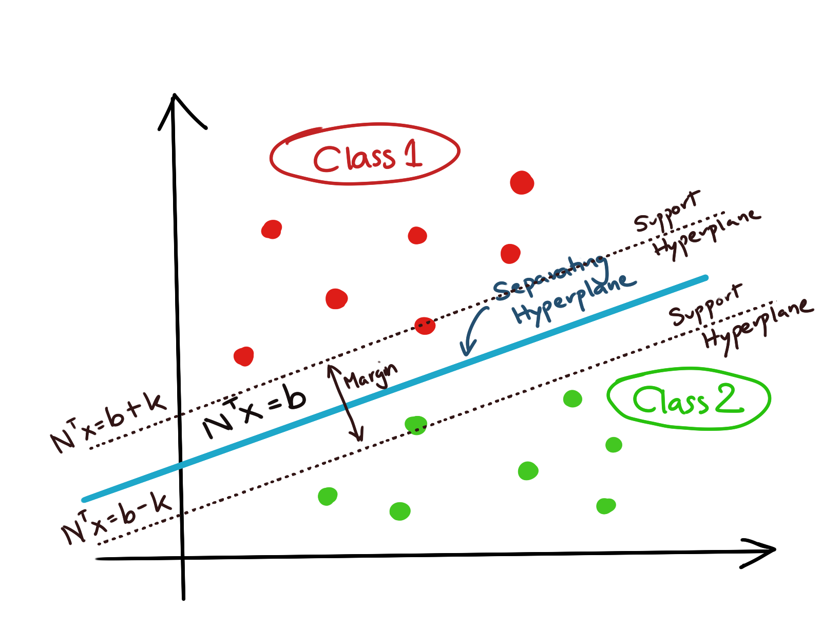
We are also given a set of training examples \(x_i, i=1,2,...,n\) which are already labelled either +1 or -1. The important assumption here is that these training data points are linearly separable, i.e., there exists a hyperplane which divides the two categories, such that no point is misclassified. Our task is to find this hyperplane with the maximum possible margin, which will be defined by its supporting hyperplanes.
Restatement of the Support Vector Machine Problem Statement
Remembering the standard form of a Quadratic Programming problem, we want the objective function to be a minimisation problem, as well as a quadratic problem.
Furthermore, we’d like to set the constant \(k=1\), and rewrite \(N\) with \(w\). Thus, the objective function may be rewritten as:
\[\mathbf{min f(x)=\frac{w^Tw}{2}}\]since squaring \(w\) does not affect the outcome of the minimisation problem.
We have two constraints; we’d like to rewrite them in the form \(g(x)\leq 0\). Thus, we get:
\[-(w^Tx_i-b)+1\leq 0, \forall x_i|y_i=+1\\ w^Tx_i-b+1\leq 0, \forall x_i|y_i=-1\]You will notice that they differ only in the sign of \((w^Tx_i-b)\), which is dependent on the reverse sign of \(y_i\). We can collapse these two inequalities into a single one by using \(y_i\) as a determinant of the sign.
\[g_i(x)=\sum_{i=1}^n-y_i(w^Tx_i-b)+1\leq 0, \forall x_i|y_i\in\{-1,+1\}\]The Lagrangian then is:
\[\mathbf{ L(w,\lambda,b)=f(x)+\lambda_i g_i(x)} \hspace{15mm}\text{(Standard Lagrangian Form)}\\ L(w,\lambda,b)=\frac{w^Tw}{2}+\sum_{i=1}^n\lambda_i [-y_i(w^Tx_i-b)+1] \\ \mathbf{ L(w,\lambda,b)=\frac{w^Tw}{2}-\sum_{i=1}^n\lambda_i [y_i(w^Tx_i-b)-1] }\]for all \(x_i\) such that \(\lambda_i\geq 0\), \(g_i(x)\leq 0\), and \(y_i\in\{-1,+1\}\).
We have already assumed the Primal and Dual Feasibility Conditions above. The Dual Optimisation Problem is then:
\[\max_\lambda\hspace{4mm}\min_{w,b} \hspace{4mm} L(w,\lambda,b)\] \[\begin{equation} \max_\lambda\hspace{4mm}\min_{w,b} \hspace{4mm} \frac{w^Tw}{2}-\sum_{i=1}^n\lambda_i [y_i(w^Tx_i-b)-1] \label{eq:lagrangian} \end{equation}\]Note that the only constraints that will be activated will be the ones which are for points lying on the supporting hyperplanes.
The Support Vector Machine Solution
We have three variables in the Lagrangian Dual: \((w,b,\lambda)\). We will now solve for each of them in turn.
1. Solving for \(w^\ast\)
Let’s see what the KKT Stationarity Condition gives us.
\[\frac{\partial L}{\partial w}=w-\sum_{i=1}^n \lambda_ix_iy_i\]Setting this partial differential to zero, we get:
\[\begin{equation} \mathbf{ w^\ast=\sum_{i=1}^n \lambda_ix_iy_i \label{eq:weight} } \end{equation}\]If we denote \(w^\ast\) as the optimal solution for \(w\).
2. Solving for \(b^\ast\)
Differentiating with respect to \(b\), and setting it to zero, we get:
\[\frac{\partial L}{\partial b}=0 \\ \Rightarrow \begin{equation} \sum_{i=1}^n \lambda_iy_i=0 \label{eq:b-constraint} \end{equation}\]This doesn’t give us an expression for \(b\) but does give us a specific condition that needs to be fulfilled by any point which lies on the supporting hyperplane.
Let us make the following observations:
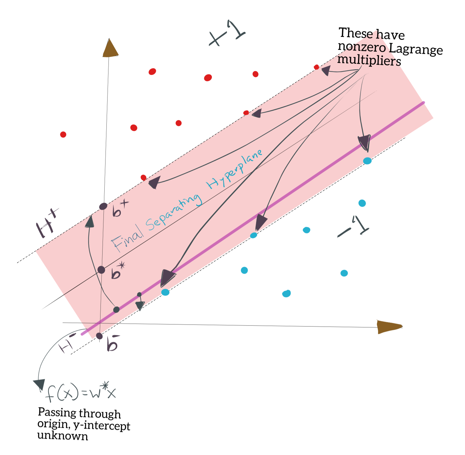
- We already know \(w^\ast\). Thus, we know the separating hyperplane through the origin, though we do not know \(b\). In two dimensions, this would be the equivalent of the y-intercept.
- For the points labelled \(+1\), the minimum value you get by plugging \(x_i\) into \(\mathbf{w^\ast x}\) is definitely a point on the (as yet undetermined) positive supporting hyperplane \(H^+\). You can have multiple points which achieve this minimum value; all of those points lie on \(H^+\), which is obviously parallel to \(f(x)=w^\ast x\).
- For the points labelled \(-1\), the maximum value you get by plugging \(x_i\) into \(\mathbf{w^\ast x}\) is definitely a point on the (as yet undetermined) negative supporting hyperplane \(H^-\). You can have multiple points which achieve this maximum value; all of those points lie on \(H^-\), which is obviously parallel to \(f(x)=w^\ast x\).
Therefore, we may find \(b^+\) and \(b^-\) by finding:
- \(H^+\) is the hyperplane with “slope” \(w^\ast\) and passing through the point \(x^+\) which gives the minimum value (positive or negative) for \(f(x)=w^\ast x\). There may be multiple points like \(x^+\); pick any one. \(H^+\) will have y-intercept \(b^+\).
- \(H^-\) is the hyperplane with “slope” \(w^\ast\) and passing through the point \(x^-\) which gives the maximum value (positive or negative) for \(f(x)=w^\ast x\). There may be multiple points like \(x^-\); pick any one. \(H^-\) will have y-intercept \(b^-\).
\(H^+\) and \(H^-\) are the supporting hyperplanes. The situation is shown below.
We already saw in Support Vector Machines from First Principles: Part One that the separating hyperplane \(H_0\) lies midway between \(H^+\) and \(H^-\), implying that \(b^\ast\) is the mean of \(b^+\) and \(b^-\). Thus, we get:
\[\begin{equation} \mathbf{ b^\ast=\frac{b^++b^-}{2} \label{eq:b} } \end{equation}\]3. Solving for \(\lambda^\ast\)
Let us simplify the \(\eqref{eq:lagrangian}\) in light of these new identities. We write:
\[L(\lambda,w^\ast,b^\ast)=\frac{w^Tw}{2}+\sum_{i=1}^n\lambda_i [y_i(w^Tx_i-b)-1] \\ =\frac{w^Tw}{2}+\sum_{i=1}^n\lambda_i y_i w^Tx_i- \sum_{i=1}^n\lambda_i y_ib + \sum_{i=1}^n\lambda_i\]The term \(\sum_{i=1}^n\lambda_i y_ib\) vanishes because of \(\eqref{eq:b-constraint}\), so we get:
\[L(\lambda,w^\ast,b^\ast)=\frac{w^Tw}{2}+\sum_{i=1}^n\lambda_i y_i w^Tx_i + \sum_{i=1}^n\lambda_i\]Applying the identity \(\eqref{eq:weight}\) to this result, we get:
\[L(\lambda,w^\ast,b^\ast)=\frac{1}{2} \sum_{i=1}^n\sum_{j=1}^n\lambda_i\lambda_jy_iy_jx_ix_j - \sum_{i=1}^n\sum_{j=1}^n\lambda_i\lambda_jy_iy_jx_ix_j + \sum_{i=1}^n \lambda_i \\ \mathbf{ L(\lambda,w^\ast,b^\ast)=\sum_{i=1}^n \lambda_i - \frac{1}{2} \sum_{i=1}^n\sum_{j=1}^n\lambda_i\lambda_jy_iy_jx_ix_j }\]Thus, \(\lambda_i\) can be solved by optimising \(L(\lambda,w^\ast,b^\ast)\), that is:
\[\lambda^\ast=\text{arginf}_\lambda L(\lambda,w^\ast,b^\ast) \\ \mathbf{ \lambda^\ast=\text{arginf}_\lambda \left[\sum_{i=1}^n \lambda_i - \frac{1}{2} \sum_{i=1}^n\sum_{j=1}^n\lambda_i\lambda_jy_iy_jx_ix_j\right] }\]Solving for \(b^\ast\): A Shortcut
I noted that to find \(b^+\) and \(b^-\), we needed to find respectively, the minimum and maximum values from each category applied to the candidate separating hyperplane \(f(x)=w^\ast x\). As it turns out, we do not need to look through all the points.
Recall that the support vectors are the ones which define the constraints in the form of supporting hyperplanes. Also, recall from our discussion on the Lagrangian Dual that the constraints are only activated for \(g(x)=0\), i.e., the Lagrange multipliers for those points are the only nonzero multipliers; all other constraints have their Lagrange multipliers as zero.
This means that if we have already computed the Lagrange multipliers, we only need to search through the points which have nonzero Lagrange multipliers to find \(b^+\) and \(b^-\). We do not need to find the maximum and minimum values, and the number of points we need to look at, is vastly reduced, presumably because most of the data points will be inside the halfspaces proper, and not exactly on the supporting hyperplanes \(H^+\) and \(H^-\).
Summary
Note that at the end of our calculation, we will have arrived at (\(\lambda^\ast\), \(w^\ast\), \(b^\ast\)) as the optimal solution for the Lagrangian. Recall that by our assumptions of Quadratic Optimisation, this Lagrangian is a concave-convex function, and thus the primal and the dual optimum solutions coincide (no duality gap). In effect, this is the same solution that we’d have gotten if we’d solved the original optimisation problem.
Once the training has completed, categorising a new point from a test set, is done simply by finding:
\[y_t=sgn[w^\ast x_t-b^\ast]\]Summarising, the expressions for the optimal Primal and Dual variables are:
\[\mathbf{ w^\ast=\sum_{i=1}^n \lambda_ix_iy_i \\ b^\ast=\frac{b^++b^-}{2} \\ \lambda^\ast=\text{arginf}_\lambda \left[\sum_{i=1}^n \lambda_i - \frac{1}{2} \sum_{i=1}^n\sum_{j=1}^n\lambda_i\lambda_jy_iy_jx_ix_j\right] }\]Relationship with the Perceptron
The Perceptron is a much simpler version of a Support Vector Machine. I’ll cover the Perceptron in its article, but simply put: the perceptron also attempts to create a linear discriminant hyperplane between two classes of data, with the purpose of classifying new data points into either one of these categories.
The form of the solution for the perceptron is also a hyperplane of the form \(f(x)=wx-b\). The perceptron may be trained sequentially, or batchwise, but regardless of the training sequence, the final adjustment that is applied to \(w\) in the hyperplane solution is proportional to \(\sum^{i=1}_n \eta x_iy_i\). This is very similar to the identity \(w^\ast=\sum_{i=1}^n \lambda_ix_iy_i\) which we derived in \(\eqref{eq:weight}\).
However, since the Perceptron does not attempt to maximise the margin between the two categories, the separating hyperplane may perform well on the training set, but might end up arbitrarily close to the support vector in either category, thus increasing the risk of misclassification of new test points in that category, which lie close to the support vector.