This is part of a series of posts breaking down the paper Plenoxels: Radiance Fields without Neural Networks, and providing (hopefully) well-annotated source code to aid in understanding.
The final code has been moved to its own repository at plenoxels-pytorch.
We continue looking at Plenoxels: Radiance Fields without Neural Networks. We set up a very contrived opacity model in our last post, which gave us an image like this:
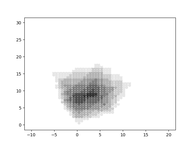
It looks very chunky; this is due to the finite resolution of the voxel world. More importantly, it does not incorporate a proper volumetric rendering model, which we will discuss in this post.
A point about performance and readability is in order here. The implementation that we are building is not going to be very fast, and the code is certainly not as optimised as it should be. However, the focus is on the explainability of the process, and how that translates into code. We may certainly delve into utilising the GPU more effectively at some point, but let us get the basics of the paper sorted first before attempting that.
Another point about cleanliness; much of the intermediate code on the way to a full implementation is going to be somewhat messy, and is presented as-is, without removing commented code, the odd print() statement and any number of variables which might not end up getting used. I’ve also always had a Python console open for really quick experiments with the PyTorch API, before lifting an expression from there and planting it in the code proper.
In this article, we will discuss the following:
- Building the Voxel Data Structure: First Pass
- Incorporating the Volumetric Rendering Model
- Incorporating Trilinear Interpolation
- Fixing Volumetric Rendering Artifacts
Building the Voxel Data Structure: First Pass
In our final model, we’d like to store opacity and the spherical harmonic coefficients per voxel. Opacity will be denoted by \(\sigma \in [0,1]\) and is as straightforward as it sounds. Let’s talk quickly about how we should encode colour. Each colour channel (R,G,B) will have its own set of 9 spherical harmonic coefficients; this gives us 27 numbers to store. Add \(\sigma\) to this, and each voxel is essentially represented by 28 numbers.
For the purposes of our initial experiments, we will not worry about the spherical harmonics, and simply represent colour using RGB triplets ranging from 0.0 to 1.0. We will still have opacity \(\sigma\). Add the three numbers necessary to represent a voxel’s position in 3D space, and we have 3+1+3=7 numbers to completely characterise a voxel.
We will begin by implementing a very simple and naive data structure to represent our world: a \((i \times j \times k)\) tensor cube. Indexing this structure using world[x,y,z] helps us locate a particular voxel in space. Each entry in this world will thus contain a tensor containing 4 numbers, the opacity \(\sigma\) and the RGB triplet.
In this article, we will not make full use of the RGB triplet; it will mostly be there for demonstration purposes before being replaced by the proper spherical harmonics model going forward.
Addressing a voxel in a position which does not exist in this world will give us \([0,0,0,0]\).
Volumetric Rendering Model
We will take a bit of a pause to understand the optical model involved in volumetric rendering since it is essential to the actual rendering and the subsequent calculation of the loss. This article follows Optical Model for Volumetric Rendering quite a bit. Solving differential equations is involved, but for the most part, you should be able to skip to the results, if you are not interested in the gory details: the relevant results are \(\eqref{eq:accumulated-transmittance}\) and \(\eqref{eq:sample-transmittance}\)
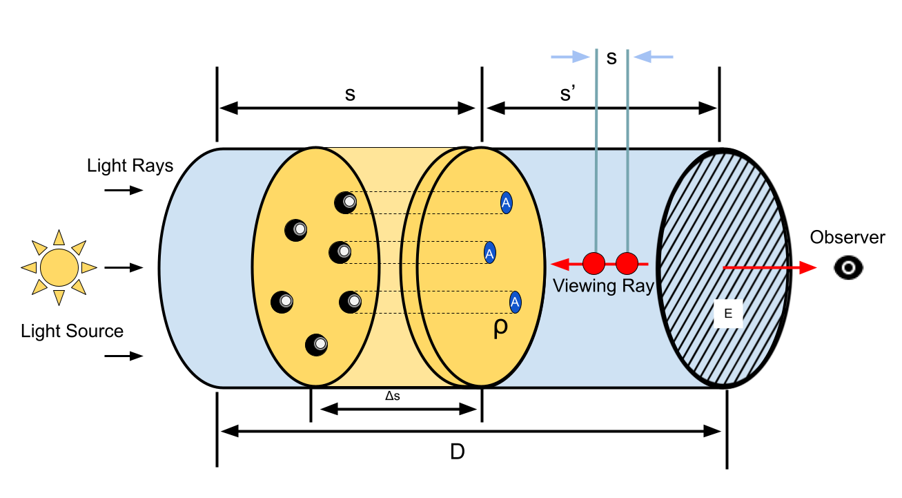
Consider a cylinder with cross-sectional area \(E\). Light flows in through the cylinder from the left. Assume a thin slab of the cylinder of length \(\Delta s\). Let \(C\) be the intensity of light (flux per unit area) entering this slab from the left. Let us assume a bunch of particles in this slab cylinder. The density of particles in this slab is \(\rho\). These particles project circular occlusions of area \(A\). If this slab is thin enough, the occlusions do not overlap.
The number of particles in this slab is then \(\rho E \Delta s\). The total area of occlusion of these particles are \(A \rho E \Delta s\). The total area of this cross section is \(E\). Thus, the fraction of light occluded is \(A \rho E \Delta s / E = A \rho \Delta s\). Then, the intensity of light exiting the slab is \(C A \rho \Delta s\).
Let us also assume that these particles emit some light, with intensity \(c\) per unit area. Then the total flux emitted is \(c A \rho E \Delta s\). The intensity (flux per unit area) is thus \(c A \rho E \Delta s / E = c A \rho \Delta s\)
Then, the delta change of intensity is:
\[\Delta C = c A \rho \Delta s - C A \rho \Delta s \\ \frac{\Delta C}{\Delta s} = c A \rho - C A \rho\]In the limit as the slab becomes infinitesmally thin, i.e., \(\Delta s \rightarrow 0\), we get:
\[\frac{dC}{ds} = c A \rho - C A \rho\]Define \(\sigma = A \rho\) to get:
\[\frac{dC}{ds} = \sigma c - \sigma C \\ \begin{equation} \frac{dC(s)}{ds} = \sigma(s) c(s) - \sigma(s) C(s) \label{eq:transmittance} \end{equation}\]Solving the Volumetric Rendering Model
This is the transmittance equation which models emission and absorption. Let’s solve it fully, so I can show you the process, even though it’s a very ordinary first-order differential equation.
Assume \(C=uv\). Then, we can write by the Chain Rule of Differentiation:
\[\frac{dC(s)}{ds} = u\frac{dv}{ds} + v\frac{du}{ds}\]Let’s get equation \(\eqref{eq:transmittance}\) into the canonical form \(Y'(x) + P(x)Y = Q(x)\).
\[\begin{equation} \frac{dC(s)}{ds} + \sigma(s)C(s) = \sigma(s)c(s) \label{eq:transmittance-canonical} \end{equation}\]The integrating factor is thus:
\[I(t) = e^{\int_0^s P(t) dt} \\ = e^{\int_0^s \sigma(t) dt}\]Multiplying both sides of \(\eqref{eq:transmittance-canonical}\) by the integrating factor, we get:
\[\frac{dC(s)}{ds}.e^{\int_0^s \sigma(t) dt} + \sigma(s)C(s).e^{\int_0^s \sigma(t) dt} = \sigma(s)c(s).e^{\int_0^s \sigma(t) dt}\]We note that for the left side:
\[\frac{d[C(s).e^{\int_0^s \sigma(t) dt}]}{ds} = \frac{dC(s)}{ds}.e^{\int_0^s \sigma(t) dt} + \sigma(s)C(s).e^{\int_0^s \sigma(t) dt}\]So we can essentially write:
\[\frac{d[C(s).e^{\int_0^s \sigma(t) dt}]}{ds} = \sigma(s)c(s).e^{\int_0^s \sigma(t) dt} \\ \int_0^D \frac{d[C(s).e^{\int_0^s \sigma(t) dt}]}{ds} ds = \int_0^D \sigma(s)c(s).e^{\int_0^s \sigma(t) dt} ds \\\]Let’s discount the constant factor of integration for the moment, and assume that \(C(0) = 0\), we then have:
\[C(D).e^{\int_0^D \sigma(t) dt} = \int_0^D \sigma(s)c(s).e^{\int_0^s \sigma(t) dt} ds \\ C(D) = \int_0^D \sigma(s)c(s).e^{\int_0^s \sigma(t) dt}.e^{-\int_0^D \sigma(t) dt} ds \\ C(D) = \int_0^D \sigma(s)c(s).e^{-\int_s^D \sigma(t) dt} ds \\ C(D) = \int_0^D \sigma(s)c(s).T'(s) ds\]Note that \(T'(s)\) is the transmittance from \(s\) to the viewer. Let’s flip the direction around so that the origin is at the viewer’s eye. Then the transmittance calculation changes from \(e^{-\int_0^{s'} \sigma'(t) dt}\) (\(\sigma'(s)\) is the opacity function as a function of \(s\) from the viewer’s eye). The integration is still from 0 to \(D\), merely in the other direction, which does not change the result. Then we get the overall colour turns out to be:
\[C(D) = \int_0^D \sigma'(s)c(s).e^{-\int_0^s \sigma'(t) dt} ds \\ T=e^{-\int_0^s \sigma'(t) dt}\]Let’s drop the subscript of \(\sigma'\), so that we get our final result.
\[\begin{equation} C(D) = \int_0^D \sigma(s)c(s).T(s) ds \\ \label{eq:volumetric-rendering-integration} \end{equation} T(s)=e^{-\int_0^D \sigma(t) dt}\]Note: I’m not sure if there is a specific mathematical procedure about how this change of coordinate is achieved. Optical Models for Volumetric Rendering uses a coordinate system which originates from the back of the volume; the previous derivations are based on that. Local and Global Illumination in the Volume Rendering Integral uses a model which uses the viewing ray starting from the viewer’s eye; that’s the model that we will start with to derive the discretised version for algorithmic implementation. Hence, the remapping.
Side Note
A very nice thing happens if \(c(s)\) happens to be constant. Let us assume it is \(c\). Then the above equation becomes:
\[C(D) = c \int_0^D \sigma(s).e^{-\int_s^D \sigma(t) dt} ds \\\]Note that from the Fundamental Theorem of Calculus (see here), we can write:
\[\frac{d[e^{-\int_s^D \sigma(t) dt}]}{ds}=e^{-\int_s^D \sigma(t) dt}.\frac{d[-\int_s^D \sigma(t) dt]}{ds} \\ = - e^{-\int_s^D \sigma(t) dt}.\frac{d[\int_s^D \sigma(t) dt]}{ds} \\ = - e^{-\int_s^D \sigma(t) dt}(\sigma(D) \frac{dD}{ds} - \sigma(s) \frac{ds}{ds}) \\ = - e^{-\int_s^D \sigma(t) dt}(\sigma(D).0 - \sigma(s).1) \\ = - e^{-\int_s^D \sigma(t) dt}(- \sigma(s)) \\ = \sigma(s).e^{-\int_s^D \sigma(t) dt} \\\]Then, we can rewrite \(C(D)\) as:
\[C(D) = c \int_0^D \frac{d[e^{-\int_s^D \sigma(t) dt}]}{ds} ds \\ = c \left[ e^{-\int_D^D \sigma(t) dt} - e^{-\int_0^D \sigma(t) dt} \right] \\ = c \left[ e^0 - e^{-\int_0^D \sigma(t) dt} \right] \\ C(D) = c \left[ 1 - e^{-\int_0^D \sigma(t) dt} \right]\]The above technique will be used to derive the discrete implementation of the integration of the transmittances along a given ray, which is what we will be using in our code.
The Discrete Volumetric Rendering Model
We still need to translate the mathematical form of the volumetric rendering model into a form suitable for implementation in code. To do this, we will have to discretise the integration procedure.
Let’s assume two samples along a ray with their distances as \(s_i\) and \(s_{i+1}\). The quantities \(c(s)\) and \(\sigma(s)\) are constant within this segment, and are denoted as \(c_i\) and \(\sigma_i\) respectively. Let the distance between these two samples be \(d_i\)Let us substitute these limits in \(\eqref{eq:volumetric-rendering-integration}\) to get:
\[C(i) = \int_{s_i}^{s_{i+1}} \sigma_i c_i.\text{exp}\left[-\int_0^s \sigma(t) dt \right] ds \\ = \sigma_i c_i \int_{s_i}^{s_{i+1}} \text{exp}\left[-\int_0^{s_i} \sigma(t) dt \right].\text{exp}\left[-\int_{s_i}^{s} \sigma(t) dt \right] ds \\ = \sigma_i c_i \int_{s_i}^{s_{i+1}} \text{exp}\left[-\int_0^{s_i} \sigma(t) dt \right].\text{exp}\left[-\int_{s_i}^{s} \sigma_i dt \right] ds \\ = \sigma_i c_i \text{exp}\left[-\int_0^{s_i} \sigma(t) dt \right] \int_{s_i}^{s_{i+1}} \text{exp}\left[-\sigma_i (s-s_i) \right] ds \\ = \sigma_i c_i \text{exp}\left[-\int_0^{s_i} \sigma(t) dt \right] \left(- \frac{1}{\sigma_i} \right) \left[ \text{exp}[-\sigma_i (s_{i+1}-s_i)] - [\text{exp}[-\sigma_i (s_i-s_i) ] \right] \\ = \sigma_i c_i \text{exp}\left[-\int_0^{s_i} \sigma(t) dt \right] \left(- \frac{1}{\sigma_i}\right) [\text{exp}\left[-\sigma_i (s_{i+1}-s_i) \right] - e^0] \\ = \sigma_i c_i \text{exp}\left[-\int_0^{s_i} \sigma(t) dt \right] \left(- \frac{1}{\sigma_i}\right) [\text{exp}\left[-\sigma_i (s_{i+1}-s_i) \right] - 1] \\ C(i) = c_i \text{exp}\left[-\int_0^{s_i} \sigma(t) dt \right] \left[1 - \text{exp}(-\sigma_i d_i)\right]\]If we denote the transparency as \(T(s) = \text{exp}\left[-\int_0^{s_i} \sigma(t) dt \right]\), we can write the above:
\[C(i) = c_i T(s_i) \left[1 - e^{-\sigma_i d_i}\right]\]Summing the above across all pairs of consecutive samples, gives us the volumetric raycasting equations \(\eqref{eq:accumulated-transmittance}\) and \(\eqref{eq:sample-transmittance}\) we will use in our actual implementation.
\[\begin{equation} \boxed{ C_i = \sum_{i=1}^N T_i \left[1 - e^{-\sigma_i d_i}\right] c_i \\ } \label{eq:accumulated-transmittance} \end{equation}\] \[\begin{equation} \boxed{ T_i = \text{exp}\left[-\sum_{i=1}^{i-1} \sigma_i d_i \right] } \label{eq:sample-transmittance} \end{equation}\]Notes
- The \(i-1\) term in the summation is so that the last pairwise distance computed is between the \((N-1)\)th and the \(N\)the sample, since there is no \((N+1)\)th sample.
- The enumeration of samples starts front to back, closer to the camera and then proceeding towards the volume.
import math
import numpy as np
import torch
import matplotlib.pyplot as plt
import functools


class Camera:
    def __init__(self, focal_length, center, basis):
        camera_center = center.detach().clone()
        transposed_basis = torch.transpose(basis, 0, 1)
        camera_center[:3] = camera_center[
                            :3] * -1  # We don't want to multiply the homogenous coordinate component; it needs to remain 1
        camera_origin_translation = torch.eye(4, 4)
        camera_origin_translation[:, 3] = camera_center
        extrinsic_camera_parameters = torch.matmul(torch.inverse(transposed_basis), camera_origin_translation)
        intrinsic_camera_parameters = torch.tensor([[focal_length, 0., 0., 0.],
                                                    [0., focal_length, 0., 0.],
                                                    [0., 0., 1., 0.]])
        self.transform = torch.matmul(intrinsic_camera_parameters, extrinsic_camera_parameters)

    def to_2D(self, point):
        # return torch.transpose(point, 0, 1)
        rendered_point = torch.matmul(self.transform, torch.transpose(point, 0, 1))
        point_z = rendered_point[2, 0]
        return rendered_point / point_z


def camera_basis_from(camera_depth_z_vector):
    depth_vector = camera_depth_z_vector[:3]  # We just want the inhomogenous parts of the coordinates

    # This calculates the projection of the world z-axis onto the surface defined by the camera direction,
    # since we want to derive the coordinate system of the camera to be orthogonal without having
    # to calculate it manually.
    cartesian_z_vector = torch.tensor([0., 0., 1.])
    cartesian_z_projection_lambda = torch.dot(depth_vector, cartesian_z_vector) / torch.dot(
        depth_vector, depth_vector)
    camera_up_vector = cartesian_z_vector - cartesian_z_projection_lambda * depth_vector

    # The camera coordinate system now has the direction of camera and the up direction of the camera.
    # We need to find the third vector which needs to be orthogonal to both the previous vectors.
    # Taking the cross product of these vectors gives us this third component
    camera_x_vector = torch.linalg.cross(depth_vector, camera_up_vector)
    inhomogeneous_basis = torch.stack([camera_x_vector, camera_up_vector, depth_vector, torch.tensor([0., 0., 0.])])
    homogeneous_basis = torch.hstack((inhomogeneous_basis, torch.tensor([[0.], [0.], [0.], [1.]])))
    homogeneous_basis[0] = unit_vector(homogeneous_basis[0])
    homogeneous_basis[1] = unit_vector(homogeneous_basis[1])
    homogeneous_basis[2] = unit_vector(homogeneous_basis[2])
    return homogeneous_basis


def basis_from_depth(look_at, camera_center):
    depth_vector = torch.sub(look_at, camera_center)
    depth_vector[3] = 1.
    return camera_basis_from(depth_vector)


def unit_vector(camera_basis_vector):
    return camera_basis_vector / math.sqrt(
        pow(camera_basis_vector[0], 2) +
        pow(camera_basis_vector[1], 2) +
        pow(camera_basis_vector[2], 2))


def plot(style="bo"):
    return lambda p: plt.plot(p[0][0], p[1][0], style)


def line(marker="o"):
    return lambda p1, p2: plt.plot([p1[0][0], p2[0][0]], [p1[1][0], p2[1][0]], marker="o")


Y_0_0 = 0.5 * math.sqrt(1. / math.pi)
Y_m1_1 = lambda theta, phi: 0.5 * math.sqrt(3. / math.pi) * math.sin(theta) * math.sin(phi)
Y_0_1 = lambda theta, phi: 0.5 * math.sqrt(3. / math.pi) * math.cos(theta)
Y_1_1 = lambda theta, phi: 0.5 * math.sqrt(3. / math.pi) * math.sin(theta) * math.cos(phi)
Y_m2_2 = lambda theta, phi: 0.5 * math.sqrt(15. / math.pi) * math.sin(theta) * math.cos(phi) * math.sin(
    theta) * math.sin(phi)
Y_m1_2 = lambda theta, phi: 0.5 * math.sqrt(15. / math.pi) * math.sin(theta) * math.sin(phi) * math.cos(theta)
Y_0_2 = lambda theta, phi: 0.25 * math.sqrt(5. / math.pi) * (3 * math.cos(theta) * math.cos(theta) - 1)
Y_1_2 = lambda theta, phi: 0.5 * math.sqrt(15. / math.pi) * math.sin(theta) * math.cos(phi) * math.cos(theta)
Y_2_2 = lambda theta, phi: 0.25 * math.sqrt(15. / math.pi) * (
        pow(math.sin(theta) * math.cos(phi), 2) - pow(math.sin(theta) * math.sin(phi), 2))


def harmonic(C_0_0, C_m1_1, C_0_1, C_1_1, C_m2_2, C_m1_2, C_0_2, C_1_2, C_2_2):
    return lambda theta, phi: C_0_0 * Y_0_0 + C_m1_1 * Y_m1_1(theta, phi) + C_0_1 * Y_0_1(theta, phi) + C_1_1 * Y_1_1(
        theta, phi) + C_m2_2 * Y_m2_2(theta, phi) + C_m1_2 * Y_m1_2(theta, phi) + C_0_2 * Y_0_2(theta,
                                                                                                phi) + C_1_2 * Y_1_2(
        theta, phi) + C_2_2 * Y_2_2(theta, phi)


def channel_opacity(position_distance_density_color_tensors):
    position_distance_density_color_vectors = position_distance_density_color_tensors.numpy()
    number_of_samples = len(position_distance_density_color_vectors)
    transmittances = list(map(lambda i: functools.reduce(
        lambda acc, j: acc + math.exp(
            - position_distance_density_color_vectors[j, 4] * position_distance_density_color_vectors[j, 3]),
        range(0, i), 0.), range(1, number_of_samples + 1)))
    density = 0.
    for index, transmittance in enumerate(transmittances):
        # if index == len(transmittances) - 1:
        #     break
        # density += (transmittance - transmittances[index + 1]) * position_distance_density_color_vectors[index, 5]
        density += transmittance * (1. -  math.exp(- position_distance_density_color_vectors[index, 4] *
                                   position_distance_density_color_vectors[index, 3])) * position_distance_density_color_vectors[index, 5]

    return density


tuples = torch.tensor([[1, 2, 3, 2, 0.2, 1, 1, 1], [1, 2, 3, 2, 0.2, 1, 1, 1]])

print(channel_opacity(tuples))

test_harmonic = harmonic(1, 2, 3, 4, 5, 6, 7, 8, 1)


class VoxelGrid:
    def __init__(self, x, y, z):
        self.grid_x = x
        self.grid_y = y
        self.grid_z = z
        self.default_voxel = torch.tensor([0.2, 0.5, 0.6, 0.7])
        self.voxel_grid = torch.zeros([self.grid_x, self.grid_y, self.grid_z, 4])

    def at(self, x, y, z):
        if self.is_outside(x, y, z):
            return torch.tensor([0., 0., 0., 0.])
        else:
            return self.voxel_grid[int(x), int(y), int(z)]

    def is_inside(self, x, y, z):
        if (0 <= x < self.grid_x and
                0 <= y < self.grid_y and
                0 <= z < self.grid_z):
            return True

    def is_outside(self, x, y, z):
        return not self.is_inside(x, y, z)

    def density(self, ray_samples_with_distances):
        collected_voxels = []
        for ray_sample in ray_samples_with_distances:
            collected_voxels.append(self.at(ray_sample[0], ray_sample[1], ray_sample[2]))
        return channel_opacity(torch.cat([ray_samples_with_distances, torch.stack(collected_voxels)], 1))

    def build_solid_cube(self):
        for i in range(self.grid_x):
            for j in range(self.grid_y):
                for k in range(self.grid_z):
                    self.voxel_grid[i, j, k] = self.default_voxel

    def build_hollow_cube(self):
        for i in range(self.grid_x):
            for j in range(self.grid_y):
                self.voxel_grid[i, j, 0] = self.default_voxel
        for i in range(self.grid_x):
            for j in range(self.grid_y):
                self.voxel_grid[i, j, self.grid_z - 1] = self.default_voxel
        for i in range(self.grid_y):
            for j in range(self.grid_z):
                self.voxel_grid[0,i,j] = self.default_voxel
        for i in range(self.grid_x):
            for j in range(self.grid_y):
                self.voxel_grid[self.grid_x - 1,i,j] = self.default_voxel
        for i in range(self.grid_z):
            for j in range(self.grid_x):
                # self.voxel_grid[j,0,i] = self.default_voxel
                self.voxel_grid[j,0,i] = torch.tensor([0.5, 0.2, 0.2, 0.2])
        for i in range(self.grid_x):
            for j in range(self.grid_y):
                self.voxel_grid[j,self.grid_y - 1,i] = self.default_voxel


grid_x = 10
grid_y = 10
grid_z = 10

world = VoxelGrid(grid_x, grid_y, grid_z)
# world.build_solid_cube()
world.build_hollow_cube()

look_at = torch.tensor([0., 0., 0., 1])
# camera_center = torch.tensor([-60., 5., 15., 1.])
# camera_center = torch.tensor([-10., -10., 15., 1.])
camera_center = torch.tensor([-20., -20., 20., 1.])
focal_length = 1

camera_basis = basis_from_depth(look_at, camera_center)
camera = Camera(focal_length, camera_center, camera_basis)

ray_origin = camera_center
camera_basis_x = camera_basis[0][:3]
camera_basis_y = camera_basis[1][:3]

camera_center_inhomogenous = camera_center[:3]

plt.rcParams['axes.facecolor'] = 'black'
plt.axis("equal")
fig1 = plt.figure()
for i in range(0, world.grid_x - 1):
    for j in range(0, world.grid_y - 1):
        for k in range(0, world.grid_z - 1):
            d = camera.to_2D(torch.tensor([[i, j, k, 1.]]))
            plt.plot(d[0][0], d[1][0], marker="o")

plt.show()
fig2 = plt.figure()
for i in np.linspace(-30, 30, 200):
    for j in np.linspace(-30, 30, 200):
        ray_screen_intersection = camera_basis_x * i + camera_basis_y * j
        unit_ray = unit_vector(ray_screen_intersection - camera_center_inhomogenous)
        density = 0.
        view_tensors = []
        for k in np.linspace(0, 100):
            ray_endpoint = camera_center_inhomogenous + unit_ray * k
            ray_x, ray_y, ray_z = ray_endpoint
            if (world.is_outside(ray_x, ray_y, ray_z)):
                continue
            # We are in the box
            view_tensors.append([ray_x, ray_y, ray_z])
            density += 0.1

        full_view_tensors = torch.unique(torch.tensor(view_tensors), dim = 0)
        if (len(full_view_tensors) <= 1):
            continue
        t1 = full_view_tensors[:-1]
        t2 = full_view_tensors[1:]
        distance_tensors = (t1 - t2).pow(2).sum(1).sqrt()
        ray_samples_with_distances = torch.cat([t1, torch.reshape(distance_tensors, (-1, 1))], 1)
        total_transmitted_light = world.density(ray_samples_with_distances)
        # print(total_transmitted_light)

        total_transmitted_light = total_transmitted_light
        if (total_transmitted_light > 1):
            total_transmitted_light = 1
        if (total_transmitted_light < 0.):
            total_transmitted_light = 0
        plt.plot(i, j, marker="o", color=str(1. - total_transmitted_light))

plt.show()
print("Done!!")
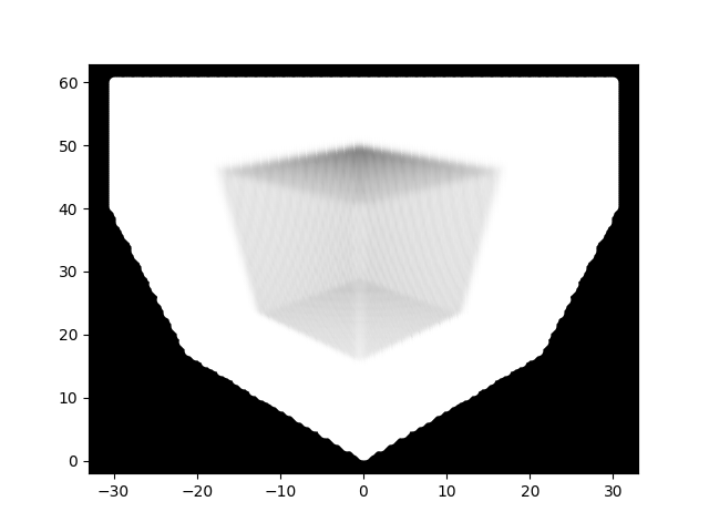
Well, that looks somewhat like a cube from the viewpoint that we chose, but it has very weird edges, as well as some very visible artifacts. This is because of the discretisation of the space and our current handling of mapping a real coordinate to voxel intensity. What we do is convert every \((x,y,z)\) to \((\text{int}(x),\text{int}(y),\text{int}(z))\), and this can assign non-zero intensities to voxels which should be empty, and vice versa.
This can be fixed by interpolating intensities of all neighbouring voxels and using the interpolated value as the voxel intensity.
Incorporating Trilinear Interpolation
In general, interpolation assigns a smoothly varying value to an intermediate point lying between two points with known values. This variation is linear when we speak of linear interpolation. Assume two points \(x_1,x_2 \in \mathbb{R}\), with \(x_1 \leq x_2\), having intensities \(c_1\) and \(c_2\) respectively. Then the colour \(c\) of any point \(x_1 \leq x \leq x_2\) can be made to vary smoothly by writing:
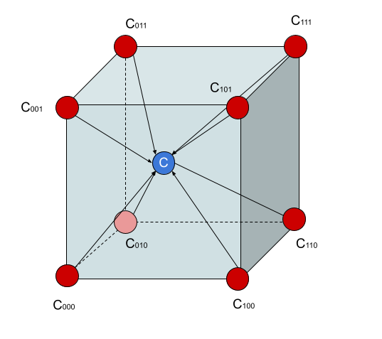
\[c(x) = c_1 + \frac{x - x_1}{x_2 - x_1} (c_2 - c_1) \\ c(x) = c_1\left(1 - \frac{x - x_1}{x_2 - x_1}\right) + \frac{x - x_1}{x_2 - x_1} c_2 \\ c(x) = c_1\left(1 - \frac{x - x_1}{x_2 - x_1}\right) + \frac{x - x_1}{x_2 - x_1} c_2 \\ c(x) = c_1(1-t) + c_2 t\]Bilinear and trilinear interpolation extends this concept to two and three dimensions. Let’s assume a point \(C(x,y,z)\). Obviously it lies in a particular voxel. We want to calculate the intensity of this voxel by interpolating the intensities of the voxels bordering its eight corners.
Let \(x_0\) be the nearest voxel ordinate to \(x\) such that \(x_0<x\). Let \(x_1\) be the nearest voxel ordinate to \(x\) such that \(x<x_1x\).
Similarly for \(y_0\), \(y_1\), \(z_0\), and \(z_1\). Then, \(C_{000}\) is the intensity of \((x_0,y_0,z_0)\). Then, \(C_{110}\) is the intensity of $$$(x_1,y_1,z_0)$, and so on.
This convention is shown below.
We use the following calculations to find the interpolated intensity of \((x,y,z)\), using the following scheme.
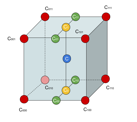
Let us define the factors \(t_x\), \(t_y\), an \(t_z\) as follows:
\[t_x = \frac{x-x_0}{x_1-x_0} \\ t_y = \frac{y-y_0}{y_1-y_0} \\ t_z = \frac{z-z_0}{z_1-z_0} \\\]Then, following calculation scheme of the diagram above, we get the following:
\[C_{00}=C_{000} (1-t_x) + C_{100} t_x \\ C_{10}=C_{010} (1-t_x) + C_{110} t_x \\ C_{01}=C_{001} (1-t_x) + C_{101} t_x \\ C_{11}=C_{011} (1-t_x) + C_{111} t_x \\ C_{0}=C_{00} (1-t_y) + C_{10} t_y \\ C_{1}=C_{01} (1-t_y) + C_{11} t_y \\ \boxed{ C=C_{0} (1-t_z) + C_{1} t_z }\]The following is the same code; instead of simply casting the coordinate to integers and addressing the voxel grid and getting the intensity of just that voxel, we now interpolate the intensity of the eight neighbouring voxels using the calculations shown above.
import math
import numpy as np
import torch
import matplotlib.pyplot as plt
import functools


class Camera:
    def __init__(self, focal_length, center, basis):
        camera_center = center.detach().clone()
        transposed_basis = torch.transpose(basis, 0, 1)
        camera_center[:3] = camera_center[
                            :3] * -1  # We don't want to multiply the homogenous coordinate component; it needs to remain 1
        camera_origin_translation = torch.eye(4, 4)
        camera_origin_translation[:, 3] = camera_center
        extrinsic_camera_parameters = torch.matmul(torch.inverse(transposed_basis), camera_origin_translation)
        intrinsic_camera_parameters = torch.tensor([[focal_length, 0., 0., 0.],
                                                    [0., focal_length, 0., 0.],
                                                    [0., 0., 1., 0.]])
        self.transform = torch.matmul(intrinsic_camera_parameters, extrinsic_camera_parameters)

    def to_2D(self, point):
        rendered_point = torch.matmul(self.transform, torch.transpose(point, 0, 1))
        point_z = rendered_point[2, 0]
        return rendered_point / point_z


def camera_basis_from(camera_depth_z_vector):
    depth_vector = camera_depth_z_vector[:3]  # We just want the inhomogenous parts of the coordinates

    # This calculates the projection of the world z-axis onto the surface defined by the camera direction,
    # since we want to derive the coordinate system of the camera to be orthogonal without having
    # to calculate it manually.
    cartesian_z_vector = torch.tensor([0., 0., 1.])
    cartesian_z_projection_lambda = torch.dot(depth_vector, cartesian_z_vector) / torch.dot(
        depth_vector, depth_vector)
    camera_up_vector = cartesian_z_vector - cartesian_z_projection_lambda * depth_vector

    # The camera coordinate system now has the direction of camera and the up direction of the camera.
    # We need to find the third vector which needs to be orthogonal to both the previous vectors.
    # Taking the cross product of these vectors gives us this third component
    camera_x_vector = torch.linalg.cross(depth_vector, camera_up_vector)
    inhomogeneous_basis = torch.stack([camera_x_vector, camera_up_vector, depth_vector, torch.tensor([0., 0., 0.])])
    homogeneous_basis = torch.hstack((inhomogeneous_basis, torch.tensor([[0.], [0.], [0.], [1.]])))
    homogeneous_basis[0] = unit_vector(homogeneous_basis[0])
    homogeneous_basis[1] = unit_vector(homogeneous_basis[1])
    homogeneous_basis[2] = unit_vector(homogeneous_basis[2])
    return homogeneous_basis


def basis_from_depth(look_at, camera_center):
    depth_vector = torch.sub(look_at, camera_center)
    depth_vector[3] = 1.
    return camera_basis_from(depth_vector)


def unit_vector(camera_basis_vector):
    return camera_basis_vector / math.sqrt(
        pow(camera_basis_vector[0], 2) +
        pow(camera_basis_vector[1], 2) +
        pow(camera_basis_vector[2], 2))


def plot(style="bo"):
    return lambda p: plt.plot(p[0][0], p[1][0], style)


def line(marker="o"):
    return lambda p1, p2: plt.plot([p1[0][0], p2[0][0]], [p1[1][0], p2[1][0]], marker="o")


Y_0_0 = 0.5 * math.sqrt(1. / math.pi)
Y_m1_1 = lambda theta, phi: 0.5 * math.sqrt(3. / math.pi) * math.sin(theta) * math.sin(phi)
Y_0_1 = lambda theta, phi: 0.5 * math.sqrt(3. / math.pi) * math.cos(theta)
Y_1_1 = lambda theta, phi: 0.5 * math.sqrt(3. / math.pi) * math.sin(theta) * math.cos(phi)
Y_m2_2 = lambda theta, phi: 0.5 * math.sqrt(15. / math.pi) * math.sin(theta) * math.cos(phi) * math.sin(
    theta) * math.sin(phi)
Y_m1_2 = lambda theta, phi: 0.5 * math.sqrt(15. / math.pi) * math.sin(theta) * math.sin(phi) * math.cos(theta)
Y_0_2 = lambda theta, phi: 0.25 * math.sqrt(5. / math.pi) * (3 * math.cos(theta) * math.cos(theta) - 1)
Y_1_2 = lambda theta, phi: 0.5 * math.sqrt(15. / math.pi) * math.sin(theta) * math.cos(phi) * math.cos(theta)
Y_2_2 = lambda theta, phi: 0.25 * math.sqrt(15. / math.pi) * (
        pow(math.sin(theta) * math.cos(phi), 2) - pow(math.sin(theta) * math.sin(phi), 2))


def harmonic(C_0_0, C_m1_1, C_0_1, C_1_1, C_m2_2, C_m1_2, C_0_2, C_1_2, C_2_2):
    return lambda theta, phi: C_0_0 * Y_0_0 + C_m1_1 * Y_m1_1(theta, phi) + C_0_1 * Y_0_1(theta, phi) + C_1_1 * Y_1_1(
        theta, phi) + C_m2_2 * Y_m2_2(theta, phi) + C_m1_2 * Y_m1_2(theta, phi) + C_0_2 * Y_0_2(theta,
                                                                                                phi) + C_1_2 * Y_1_2(
        theta, phi) + C_2_2 * Y_2_2(theta, phi)


def channel_opacity(position_distance_density_color_tensors):
    position_distance_density_color_vectors = position_distance_density_color_tensors.numpy()
    number_of_samples = len(position_distance_density_color_vectors)
    transmittances = list(map(lambda i: functools.reduce(
        lambda acc, j: acc + math.exp(
            - position_distance_density_color_vectors[j, 4] * position_distance_density_color_vectors[j, 3]),
        range(0, i), 0.), range(1, number_of_samples + 1)))
    density = 0.
    for index, transmittance in enumerate(transmittances):
        # if index == len(transmittances) - 1:
        #     break
        # density += (transmittance - transmittances[index + 1]) * position_distance_density_color_vectors[index, 5]
        density += transmittance * (1. - math.exp(- position_distance_density_color_vectors[index, 4] *
                                                  position_distance_density_color_vectors[index, 3])) * \
                   position_distance_density_color_vectors[index, 5]

    return density


tuples = torch.tensor([[1, 2, 3, 2, 0.2, 1, 1, 1], [1, 2, 3, 2, 0.2, 1, 1, 1]])

print(channel_opacity(tuples))

test_harmonic = harmonic(1, 2, 3, 4, 5, 6, 7, 8, 1)


class VoxelGrid:
    def __init__(self, x, y, z):
        self.grid_x = x
        self.grid_y = y
        self.grid_z = z
        self.default_voxel = torch.tensor([0.005, 0.5, 0.6, 0.7])
        self.voxel_grid = torch.zeros([self.grid_x, self.grid_y, self.grid_z, 4])

    def at(self, x, y, z):
        if self.is_outside(x, y, z):
            return torch.tensor([0., 0., 0., 0.])
        else:
            return self.voxel_grid[int(x), int(y), int(z)]

    def is_inside(self, x, y, z):
        if (0 <= x < self.grid_x and
                0 <= y < self.grid_y and
                0 <= z < self.grid_z):
            return True

    def is_outside(self, x, y, z):
        return not self.is_inside(x, y, z)

    def density(self, ray_samples_with_distances):
        collected_voxels = []
        for ray_sample in ray_samples_with_distances:
            x = ray_sample[0]
            y = ray_sample[1]
            z = ray_sample[2]
            x_0, x_1 = int(x), int(x) + 1
            y_0, y_1 = int(y), int(y) + 1
            z_0, z_1 = int(z), int(z) + 1
            x_d = (x - x_0) / (x_1 - x_0)
            y_d = (y - y_0) / (y_1 - y_0)
            z_d = (z - z_0) / (z_1 - z_0)
            c_000 = self.at(x_0, y_0, z_0)
            c_001 = self.at(x_0, y_0, z_1)
            c_010 = self.at(x_0, y_1, z_0)
            c_011 = self.at(x_0, y_1, z_1)
            c_100 = self.at(x_1, y_0, z_0)
            c_101 = self.at(x_1, y_0, z_1)
            c_110 = self.at(x_1, y_1, z_0)
            c_111 = self.at(x_1, y_1, z_1)
            c_00 = c_000 * (1 - x_d) + c_100 * x_d
            c_01 = c_001 * (1 - x_d) + c_101 * x_d
            c_10 = c_010 * (1 - x_d) + c_110 * x_d
            c_11 = c_011 * (1 - x_d) + c_111 * x_d

            c_0 = c_00 * (1 - y_d) + c_10 * y_d
            c_1 = c_01 * (1 - y_d) + c_11 * y_d

            c = c_0 * (1 - z_d) + c_1 * z_d
            # print(c)
            # collected_voxels.append(self.at(ray_sample[0], ray_sample[1], ray_sample[2]))
            collected_voxels.append(c)
        return channel_opacity(torch.cat([ray_samples_with_distances, torch.stack(collected_voxels)], 1))

    def build_solid_cube(self):
        for i in range(self.grid_x):
            for j in range(self.grid_y):
                for k in range(self.grid_z):
                    self.voxel_grid[i, j, k] = self.default_voxel

    def build_hollow_cube(self):
        for i in range(10, self.grid_x - 10):
            for j in range(10, self.grid_y - 10):
                self.voxel_grid[i, j, 9] = self.default_voxel
        for i in range(10, self.grid_x - 10):
            for j in range(10, self.grid_y - 10):
                self.voxel_grid[i, j, self.grid_z - 1 - 10] = self.default_voxel
        for i in range(10, self.grid_y - 10):
            for j in range(10, self.grid_z - 10):
                self.voxel_grid[9, i, j] = self.default_voxel
        for i in range(10, self.grid_x - 10):
            for j in range(10, self.grid_y - 10):
                self.voxel_grid[self.grid_x - 1 - 10, i, j] = self.default_voxel
        for i in range(10, self.grid_z - 10):
            for j in range(10, self.grid_x - 10):
                self.voxel_grid[j, 9, i] = self.default_voxel
        for i in range(10, self.grid_x - 10):
            for j in range(10, self.grid_y - 10):
                self.voxel_grid[j, self.grid_y - 1 - 10, i] = self.default_voxel


grid_x = 40
grid_y = 40
grid_z = 40

world = VoxelGrid(grid_x, grid_y, grid_z)
# world.build_solid_cube()
world.build_hollow_cube()

look_at = torch.tensor([0., 0., 0., 1])
# camera_center = torch.tensor([-60., 5., 15., 1.])
# camera_center = torch.tensor([-10., -10., 15., 1.])
camera_center = torch.tensor([-20., -20., 40., 1.])
focal_length = 1

camera_basis = basis_from_depth(look_at, camera_center)
camera = Camera(focal_length, camera_center, camera_basis)

ray_origin = camera_center
camera_basis_x = camera_basis[0][:3]
camera_basis_y = camera_basis[1][:3]

camera_center_inhomogenous = camera_center[:3]

plt.rcParams['axes.facecolor'] = 'black'
plt.axis("equal")
fig1 = plt.figure()
for i in range(0, world.grid_x):
    for j in range(0, world.grid_y):
        for k in range(0, world.grid_z):
            voxel = world.at(i, j, k)
            if (voxel[0] == 0.):
                continue
            d = camera.to_2D(torch.tensor([[i, j, k, 1.]]))
            plt.plot(d[0][0], d[1][0], marker="o")

plt.show()
fig2 = plt.figure()
for i in np.linspace(-30, 30, 200):
    for j in np.linspace(-10, 60, 200):
        ray_screen_intersection = camera_basis_x * i + camera_basis_y * j
        unit_ray = unit_vector(ray_screen_intersection - camera_center_inhomogenous)
        density = 0.
        view_tensors = []
        # To remove artifacts, set ray step samples to be higher, like 200
        for k in np.linspace(0, 100, 100):
            ray_endpoint = camera_center_inhomogenous + unit_ray * k
            ray_x, ray_y, ray_z = ray_endpoint
            if (world.is_outside(ray_x, ray_y, ray_z)):
                continue
            # We are in the box
            view_tensors.append([ray_x, ray_y, ray_z])
            density += 0.1

        full_view_tensors = torch.unique(torch.tensor(view_tensors), dim=0)
        if (len(full_view_tensors) <= 1):
            continue
        t1 = full_view_tensors[:-1]
        t2 = full_view_tensors[1:]
        distance_tensors = (t1 - t2).pow(2).sum(1).sqrt()
        ray_samples_with_distances = torch.cat([t1, torch.reshape(distance_tensors, (-1, 1))], 1)
        total_transmitted_light = world.density(ray_samples_with_distances)
        # print(total_transmitted_light)

        total_transmitted_light = total_transmitted_light
        if (total_transmitted_light > 1):
            total_transmitted_light = 1
        if (total_transmitted_light < 0.):
            total_transmitted_light = 0
        plt.plot(i, j, marker="o", color=str(1. - total_transmitted_light))

plt.show()
print("Done!!")
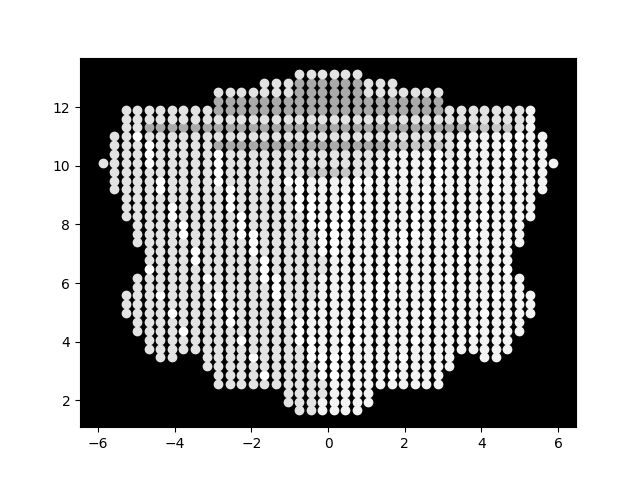
Here is the result.
As you can, see, it clearly looks like a proper cube, with none of the lumpy borders we saw in the previous code example. However, there is still some banding that is evident. Our next code sample fixes that.
Fixing Volumetric Rendering Artifacts
Common Artifacts in Volume Rendering calls the kind of artifacts we see “onion rings”. The solution they propose is to increase the sampling rate, which we change from 100 to 200.
This is the result.
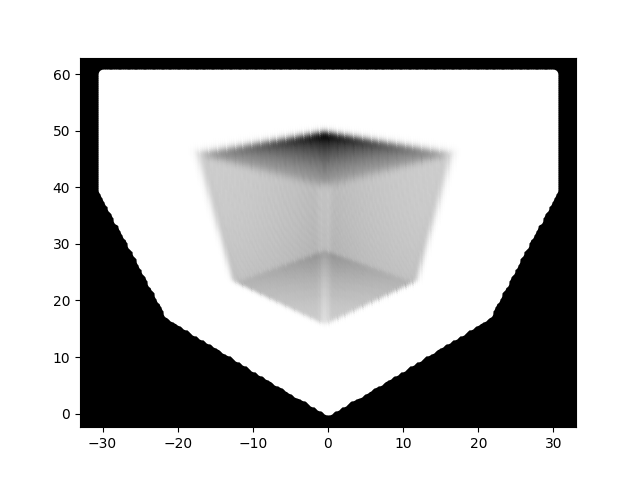
As you can see, the rings are more or less gone.
This concludes the second part of implementing the Plenoxels paper. We will tackle integrating the spherical harmonics into our model in the sequel.