Plenoxels and Neural Radiance Fields using PyTorch: Part 6

Avishek Sen Gupta on 27 December 2022

---

This is part of a series of posts breaking down the paper Plenoxels: Radiance Fields without Neural Networks, and providing (hopefully) well-annotated source code to aid in understanding.

The final code has been moved to its own repository at plenoxels-pytorch.

• Part 1
• Part 2
• Part 3
• Part 4
• Part 5
• Part 6 (this one)

We continue looking at Plenoxels: Radiance Fields without Neural Networks. In this sequel, we address some remaining aspects of the paper, before concluding with our study of this paper. We specifically consider the following:

Note: We leave this post open-ended, and will append to/modify it as we obtain further results.

• Voxel pruning: This will probably require us to modify our core data structure to be a little more efficient, because it will involve storing all the transmittances of the entire training set per epoch, and then zeroing out candidate voxels.
• Encouraging voxel sparsity: Adding more regularisation terms will encourage sparsity of voxels. In the paper, the Cauchy loss is incorporated to speed up computations.
• Coarse-to-fine resolution scaling: This will be needed to better resolve the fine structure of our training scenes. At this point, we are working with a very coarse low resolution of \(40 \times 40 \times 40\). We can get higher resolutions than this, but this will need more work, and more computations.

The code for this article can be found here: Volumetric Rendering Code with TV Regularisation

Demonstration on a real world dataset

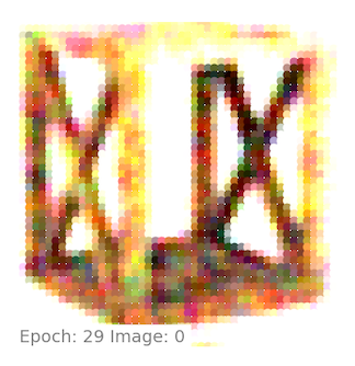
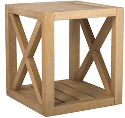
For our field-testing we pick a model from the Amazon Berkeley Objects dataset. The ABO Dataset is made available under the Creative Commons Attribution-NonCommercial 4.0 International Public License (CC BY-NC 4.0), and is available here.

We have picked 72 views of a full \({360}^\circ\) fly-around of the object, and run it through our code. We demonstrate the learning using a single training for the image. We will show more results as they become available.

Notes on the Code

1. Fixing a Transmittance calculation bug

We derived the transmittance and the consequent colour values as the following:

\[\begin{equation} \boxed{ C_i = \sum_{i=1}^N T_i \left[1 - e^{-\sigma_i d_i}\right] c_i \\ } \label{eq:accumulated-transmittance} \end{equation}\] \[\begin{equation} \boxed{ T_i = \text{exp}\left[-\sum_{i=1}^{i-1} \sigma_i d_i \right] } \label{eq:sample-transmittance} \end{equation}\]

Unfortunately the implementation had a bug where \(T_i=-\sum_{i=1}^{i-1} \text{exp } (\sigma_i d_i)\). This gave us increasing transmittance with distance. We fixed that in this implementation, so that transmittance is calculated correctly.

2. Refactoring volumetric rendering to use matrices instead of loops

Instead of looping over samples in a particular ray to calculate transmittances and consequent colour values, we refactored the code to use a more matrix approach.

The equation \(\eqref{eq:sample-transmittance}\) can be written for all \(T_i\) as:

\[T = \text{exp} (-{(\Sigma \odot \Delta)}^T S)\]

where \(\odot\) denotes the Hadamard Product (element-wise product), and the other terms are as follows:

\[T = \begin{bmatrix} T_1 && T_1 && \vdots && T_N \end{bmatrix} \\ \Sigma = \begin{bmatrix} \sigma_1 \\ \sigma_1 \\ \vdots \\ \sigma_N \end{bmatrix}, \Delta = \begin{bmatrix} \delta_1 \\ \delta_1 \\ \vdots \\ \delta_N \end{bmatrix}, \\ S = \begin{bmatrix} 1 && 1 && 1 && \ldots && 1 \\ 0 && 1 && 1 && \ldots && 1 \\ 0 && 0 && 1 && \ldots && 1 \\ \vdots && \vdots && \vdots && && \vdots \\ 0 && 0 && 0 && \ldots && 1 \end{bmatrix}\]

We call \(S\) the summing matrix. Similarly, the colour \(C_i\) for all samples in a ray, can be calculated as:

\[C = T.(I' - \text{exp }(- \Sigma \odot \Delta))\]

where \(I'\) is an \(n \times 1\) matrix, like so:

\[I'= \begin{bmatrix} 1 \\ 1 \\ \vdots \\ 1 \end{bmatrix}\]

These give us the matrix forms for the volumetric rendering calculations.

\[\begin{equation} \boxed{ C = T.(I' - \text{exp }(- \Sigma \odot \Delta)) \\ T = \text{exp} (-{(\Sigma \odot \Delta)}^T S) } \label{eq:volumetric-formula-matrix} \end{equation}\]

3. Configuring empty voxels to be light or dark

Some sets of training images have their background as white, some as dark. We make this configurable by introducing the EMPTY object, which can be configured to be either black or white, depending upon the training and rendering situation.

Adding the pruned attribute

We add the pruned attribute to voxels. This prevents a voxel parameter from being activated, as well as sets its opacity and spherical harmonic coefficients to zero.

Allowing the world to scale up

A scale parameter is introduced in the world; this represents the scale of the voxel in relation to the world itself. A scale of 1, means that a voxel is the same as a unit cube in the world. The world can now scale; this is done through the scale_up() function. The voxel dimensions are doubled, the scale is reduced, and the original voxel is replicated to its newly-spawned 7 neighbours; see the diagram below for an explanation.

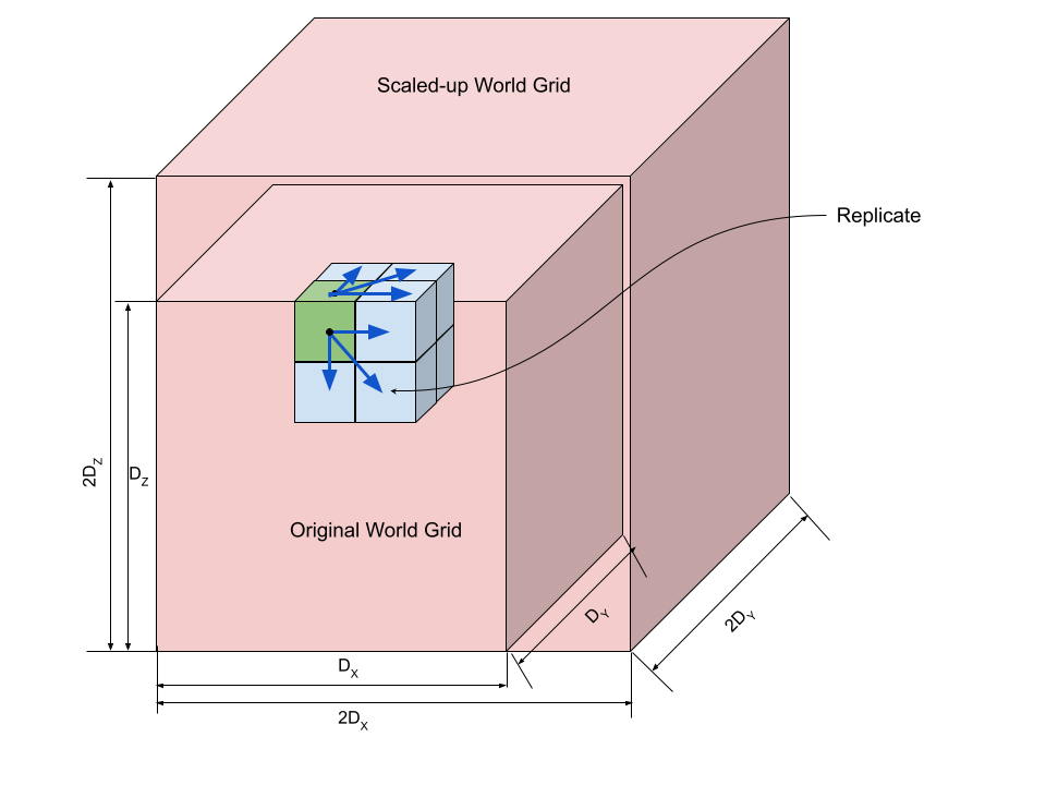
Note that though the grid size doubles, the size of the world stays the same; in effect, the voxels halve in each dimension.

Cauchy Regularisation

The Cauchy Loss Function is introduced in the paper Robust subspace clustering by Cauchy loss function. The Cauchy Loss function in the Plenoxels paper is given as:

\[\Delta_C = \lambda_C \sum_{i,k} \text{log}_e (1 + 2 \sigma{(r_i(t_k))}^2)\]

Essentially, we sum up the opacity of all samples in a training ray, over all our training rays. Let us explain the rationale for why the Cauchy Loss Function is a good sparsity prior.

TODO: Explain why CLF is used as a sparsity prior.

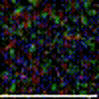
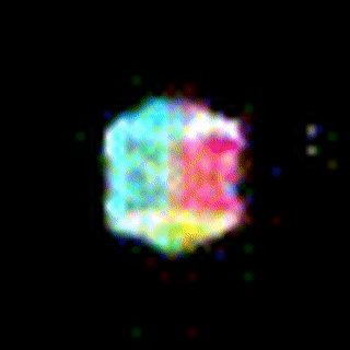
Reconstruction without Cauchy Regularisation

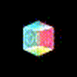
Reconstruction with Cauchy Regularisation

Conclusion

This concludes our study of the Plenoxels paper. There is a lot more scope for fine-tuning, but on the whole this survey covers the important aspects. It is a lovely paper, and is a good example of what can be accomplished without resorting directly to Neural Networks.

References

• Amazon Berkeley Objects Dataset
• Plenoxels: Radiance Fields without Neural Networks
• Plenoxels Explained
• Robust subspace clustering by Cauchy loss function

---