Plenoxels and Neural Radiance Fields using PyTorch: Part 4

Avishek Sen Gupta on 18 December 2022

---

This is part of a series of posts breaking down the paper Plenoxels: Radiance Fields without Neural Networks, and providing (hopefully) well-annotated source code to aid in understanding.

The final code has been moved to its own repository at plenoxels-pytorch.

• Part 1
• Part 2
• Part 3
• Part 4 (this one)
• Part 5
• Part 6

We continue looking at Plenoxels: Radiance Fields without Neural Networks. We have built our volumetric renderer; it is now time to start calculating loss from training images. We start off with trying out some test images, the source of which will be our renderer itself, as a kind of control set.

The code for this article can be found here: Volumetric Rendering Code

Before we begin however, let’s talk quickly about some technical details of the code.

Technical Comments on the Code

1. How is the camera basis calculated?

We wanted to simplify our calculations for creating the camera coordinate system. Usually, you’d be given a camera basis or a camera transformation matrix explicitly. To make it easier to generate scenes and not worry about having to calculate an orthogonal basis by hand every time, our camera simply uses two parameters: the look_at and camera_center parameters. Together, these immediately give us a vector which points in the direction that the camera is looking, which is the Z-axis in the camera’s system.

We now need to generate two orthogonal vectors from this to complete the coordinate system. First, we need to define the “up-vector”. In most situations, we want the camera to be upright; loosely, the world’s Z-axis should always be up.

In the calculation below, \(x_c\), \(y_c\), and \(z_c\) represent the three basis vectors of the camera, and \(z_w\) represents the world’s Z-axis.

\[z_c.y_c = 0 \\ y_c + \lambda z_c = z_w\]

We need to find \(y_c\). We can simply deduce from the above that:

\[z_c.(z_w - \lambda z_c) = 0 \\ z_c.z_w - \lambda z_c.z_c = 0 \\ \lambda = \frac{z_c.z_w}{z_c.z_c} = \frac{z_c.z_w}{ {|z_c|}^2}\]

Then we can write \(y_c\) as:

\[y_c = z_w - \frac{z_c.z_w}{ {|z_c|}^2} z_w\]

This is what the first part of the camera_basis_from() function does. Now that we have two axes, the third axis can be calculated by simply taking the cross product of \(z_c\) and \(y_c\) to get \(x_c\). Thus, \((x_c, y_c, z_c)\) constitute an orthogonal basis for the camera, with \(z_c\) pointing in the direction where the camera is looking.

The calculation is depicted in the figure below.

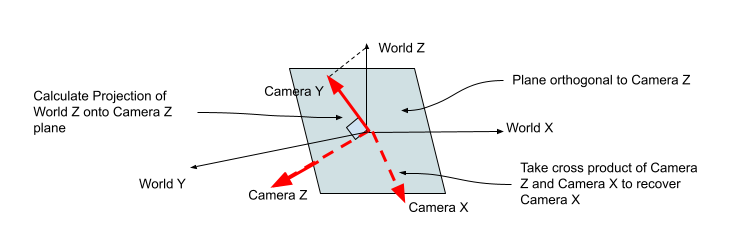
Note that we also normalise these vectors to unit length before returning the basis.

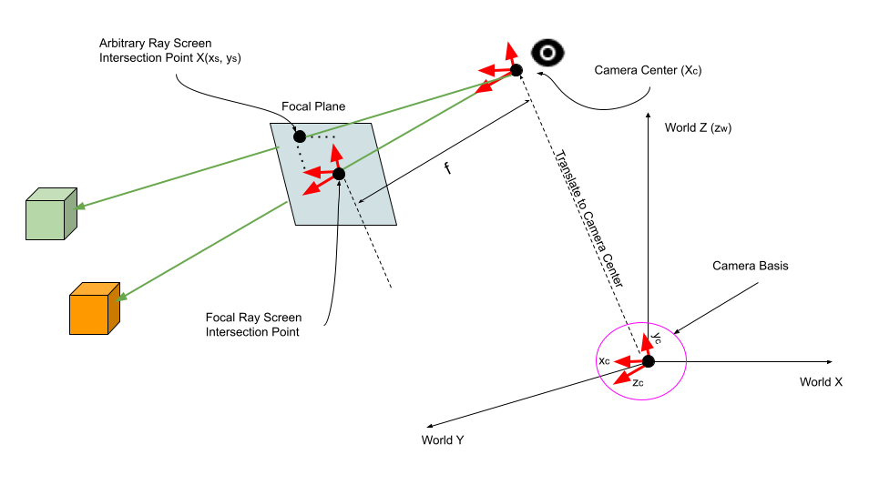
2. How are the rays on screen calculated?

We have seen above how to calculate the camera basis. We need to now calculate where the focal plane is, because the viewing rays originating from the camera will intersect this plane. In fact, this plane will be important in deciding which viewing rays to actually fire. The normal to the focal plane is instantly given by \(z_c\), the camera’s Z-axis. We want to render everything which is within the bounds of the focal plane screen. This in turn depends upon the length and height of the screen. We can pick any dimension: in the code, we have chosen a square of size \([-1, 1] \times [-1, 1]\), with a resolution of 100 samples in each direction.

For each of these points \((x_s,y_s)\), we want to translate from \({\mathbb{R}}^2 \in [0,1] \times [0,1]\) into world coordinates. This is done by simply scaling the camera’s unit basis vectors \(x_c\) and \(y_c\) by the corresponding amounts.

One last thing remains: to translate this result to the actual focal plane, because the camera’s basis (any basis, for that matter of fact) is centered at \((0,0,0)\). For this we need the coordinates of the focal point. This is done by simply scaling the unit basis vector \(z_c\) by the focal length of the camera, and translating the result to the camera center \(X_c\). The calculation is summarised below: keep in mind that \(f\), \(x_s\), and \(y_s\) are scalars.

\[X(x_s,y_s) = x_s.x_c + y_s.y_c + (f.z_c + X_c)\]

The calculation is visualised in the diagram below.

3. How are the RGB values calculated from the spherical harmonics?

In the code, the convention is to use a scale of \([0.0, 1.0]\) for each colour channel. Depending upon the coefficients and the number of ray samples, the calculated colour of any point in the view screen can routinely lie outside \([0,1]\). The paper does not elaborate much on how to clamp these values, beyond using a ReLU for linearity. However, the original NERF paper uses a sigmoid function, which restricts everything to \([0.0, 1.0]\), which is what we use here. It’s easy to implement, differentiable, and gives good results.

Refactoring the Data Structure

In preparation for making our data structures more flexible, as well as making the structures more amenable for PyTorch’s optimisation routines, we will need refactor our data structure. So far, we have simply used a simple 3D tensor, whose elements represent the voxels. We will continue to maintain this structure for now, but we will introduce a more pointer based structure to easily reference and store the voxels that our viewing rays actually intersect during each training cycle, because those are the only parameters that we will be optimising every time we train; the other voxel values are frozen.

The renderer will thus need refactoring; however, we will continue to use the original renderer to generate ground truth that we can use to validate that the refactored renderer still generates correct images.

The new data structure is shown below; the structure of one viewing ray is elaborated in this diagram.

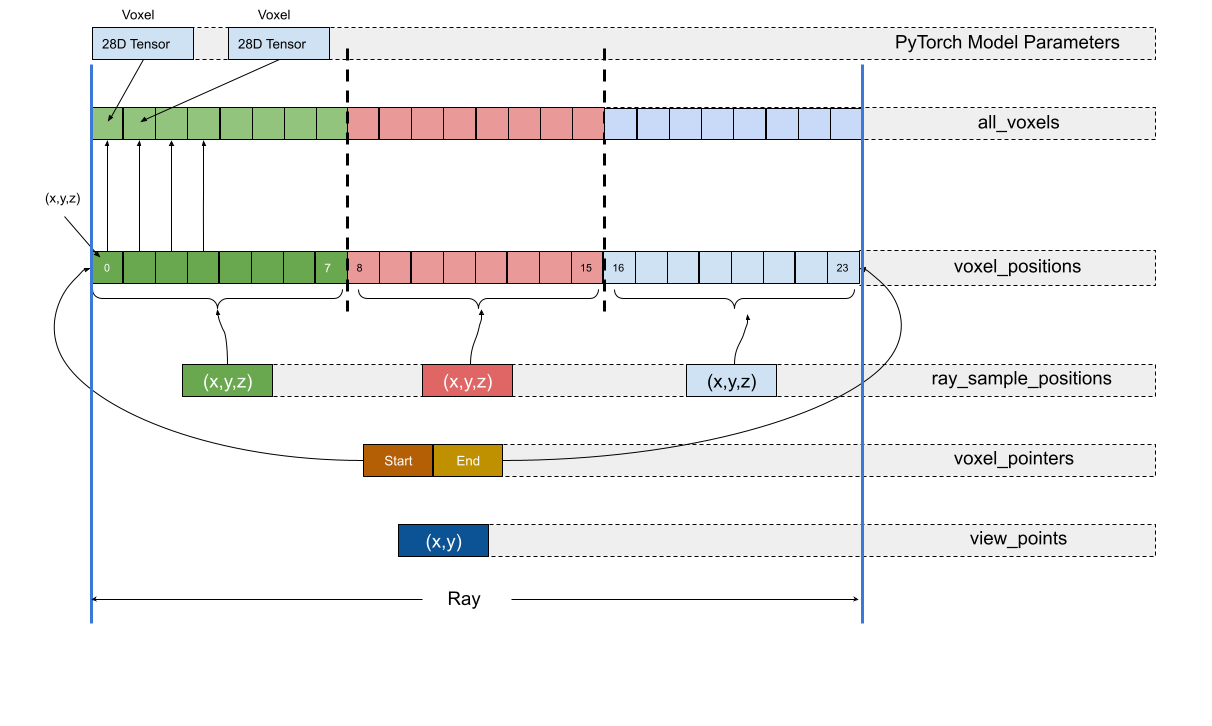
Here is a quick explanation of the structures involved.

• view_points: These represent each point on the screen that will actually be rendered, and thus are represented by \((x,y)\) pairs. Each point ultimately corresponds to one viewing ray.
• ray_sample_positions: Volumetric rendering requires sampling the voxels at specific samples along the ray. This structure contains a flat list of all these sample positions along all rays. The start and end sample of a given ray is located using the voxel_pointers structure.
• voxel_positions: For each ray sample, the 8 neighbouring voxels have their coefficients interpolated to yield the coefficients for that sample. Thus, each sample has 8 voxels; if there are \(n\) ray samples i a ray, there are \(8n\) voxels in that way. All the voxel positions of all the rays are stored in this data structure.
• voxel_pointers: The indices of the start voxel and the end voxel of each ray are stored i each entry of this data structure. Using this, we can reference any voxel group for any sample given the index \(i\) of the sample. Each entry here is a (start, end) tuple, corresponding to one ray.
• all_voxels: Each entry here is a voxel tensor containing the opacity and the 27 spherical harmonic coefficients. There is an ordered 1:1 correspondence between each entry here and the voxel_positions structure.

So far, our renderer has simply iterated over a contiguous rectangular area and rendered each point in that area. For training, we will select a stochastic set of rays (5000 in the paper, about 500-1000 in our implementation) and use those to calculate the loss. Thus, our renderer should be prepared to render only specific rays. Some refactoring on this front is also done.

Incorporating A Single Training Image

Let’s test the optimisation on images generated with the exact renderer which will be used in training. The training scheme is as follows:

• We use only one training image for demonstration.
• The initial world is filled with voxels with random opacities and spherical harmonic coefficients between 0 and 1.
• PlenoxelModel is our custom PyTorch model. This will hold our parameters. These parameters are essentially a flat list of voxels which are intersected by about 1000 viewing rays. The parameters to be optimised are the opacity and the 27 spherical harmonic coefficients in each voxel.
• We train for 3-5 epochs with a low learning rate of around 0.001 on the same image for the same set of voxels. Yes, this is not what we will end up with, but it’s a simple starting point.
• The mean squared error for each channel is calculated and summed up across channels. This gives us the total MSE. We will add in the Total Variance regularisation later.

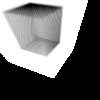
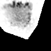
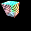
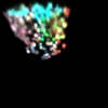
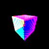
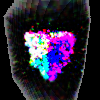
Reconstruction Results

These are using just one image, and the reconstruction is correct only from that specific viewpoint.

Debugging Tips

There is one thing that we should also address: the code as it is, had some bugs that resulted in the rendering looking wonky from certain angles, and not working at all from other angles. Sometimes bugs may not become apparent till much later; having said that, here are some debugging tips I found helpful. Note that most, if not all, of these are general practices when you are trying to debug any code, not just ML code. These become especially important, though, when you are debugging a rendering error which involves thousands of pixels.

• Find the simplest program which can reproduce the issue, preferably in a self-contained code fragment: This is what we had to do when puzzling over why the optimisation wasn’t actually updating any of the parameters. Whittling down the entire code to about 70 lines of isolated code helped identify the problem by comparing it with toy examples which were already working. The code for reproducing that particular bug can be found here.
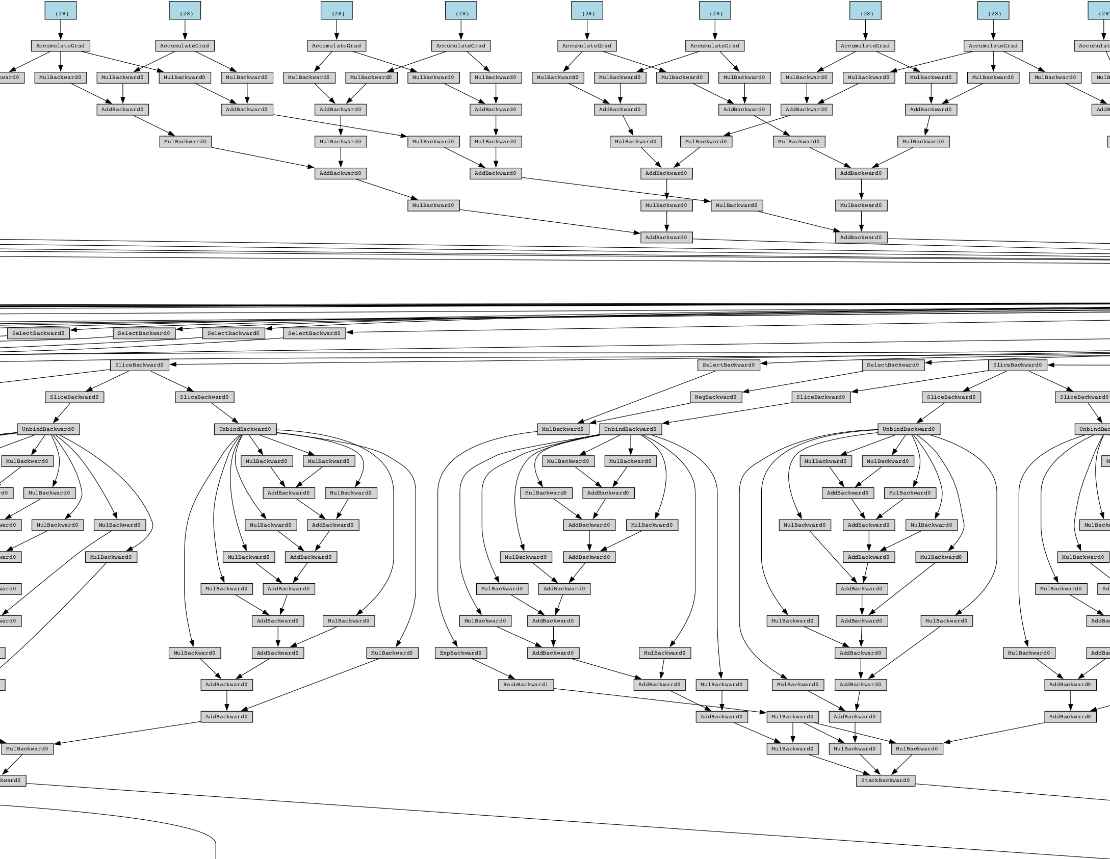
• Track gradient function propagation throughout calculations: This is the easiest, but messy, way of pinpointing where your gradient propagation breaks. Log the output tensor at each stage; if you don’t see a grad_fn in the tensor description, or simply something like tensor(XXX., requires_grad=True) in the middle of your calculations, go back to the previous step and see which calculation was not done using PyTorch’s APIs. In particular, do not wrap outputs using torch.tensor(...).
• Check gradient propagation graph using PyTorchViz: This can be prohibitively mind-boggling if you are trying to make sense of the entire graph when your code is not a toy example; for example, see below for the renderer graph at one stage of my debugging. It can be useful to make sure that all your computations are included in the chain and that it’s not broken somewhere in the middle.

• For loops, reduce it to a single degenerate / problematic value and trace: This is especially pertinent when you are rendering hundreds (if not thousands) of rays, and your rendering is not correct. Reduce it to a degenerate case: loop once with a known camera position that you can visualise easily using pen and paper, and log ray intersections, skipped voxels, and transmittance values. More often than not, you will be able to find the problem almost immediately after seeing the output. This helped me fix a bug where some randomly-initialised voxels were not rendering: I realised that some of the random spherical harmonic coefficients yielded negative RGB values, which were then clamped down very close to zero.
• Beware of divide-by-zero errors: A simple example is calculating the viewing angles of the camera given its Cartesian coordinates. This involves converting to spherical coordinates. If the viewing angles happen to align with some of the Cartesian basis vectors, the denominator in some of these calculations becomes zero, and you get \(nan\).
• Before refactoring complicated rendering logic, have a ground truth version at all times to check your refactored work: This is very useful when performing a refactoring where you might make mistake at any point, and need a reference to check your ongoing work.

Conclusion

We have come quite far in our implementation of the paper. We will progress to training using multiple training images in the sequel and (probably) add TV regularisation.

References

• Plenoxels: Radiance Fields without Neural Networks
• Plenoxels Explained
• How to use Pytorch as a general optimizer

---