Plenoxels and Neural Radiance Fields using PyTorch: Part 1

Avishek Sen Gupta on 4 December 2022

This is part of a series of posts breaking down the paper Plenoxels: Radiance Fields without Neural Networks, and providing (hopefully) well-annotated source code to aid in understanding.

The final code has been moved to its own repository at plenoxels-pytorch.

The relevant paper is Plenoxels: Radiance Fields without Neural Networks. We will also use this explanation to understand some parts of this paper a little better.

Before we get into the implementations of the paper proper, we will need a game plan. This game plan will include some theoretical background that we will have to go through to implement parts of this paper. The theoretical background will include:

Camera Model
Volumetric Rendering Model
Spherical Harmonics
Regularisation

In this specific post, however, we will start building out a simple volumetric renderer. On the way, we will also discuss the pinhole camera model, on which most of our rendering will be based on.

The World Camera Model and some Linear Algebra

The pinhole camera model has the following characteristics.

The model exists in the world, and is expressed in the world coordinate system. This is usually our default three-dimensional basis.
The camera exists somewhere in the world, and has its own coordinate system, the camera coordinate system. This is characterised by the location of the camera, the focal length of the camera, and the three-dimensional basis for the camera.
The screen of the camera (which is basically where the image is formed) has its own two-dimensional coordinate system.

Camera World Mode

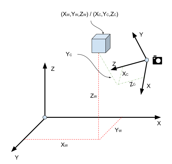
The challenge is this: we have a point in 3D space expressed in the world coordinate system, let’s call it \(X_W\); we want to know what this point will translate to on the 2D coordinate system of the camera screen/film. At a very high level, given all the information about the camera and the world, we want to know about the camera transform matrix \(P\).

\[\begin{equation} X_V=TX_W \label{eq:1} \end{equation}\]

In the above diagram \(X_W = (x_w, y_w, z_w)\). We need to do the following steps:

Express \(X_W\) in the coordinate system of the camera as \(X_C\). These are the extrinsic parameters of the camera.
Express \(X_C\) in the coordinate system of the camera screen, taking into account focal length. These are the intrinsic parameters of the camera.

The camera is characterised first by the camera center \(C\). The first step is translating the entire world so that the origin is now at the camera. This is simply done by calculating \(X_W-C\).

The camera is also characterised by its basis, which is essentially three 3D vectors. Now that the camera is at the center, we need to rotate the world so that everything in it is expressed using the camera’s coordinate system. How do we achieve this change of basis?

We have discussed change of basis before in a few articles. Specifically see The Gram-Schmidt Orthogonalisation and Geometry of the Multivariate Gaussian Distribution.

Specifically, we have an arbitrary basis \(B\) in \(n\)-dimensional space, and let there be a vector \(v\) expressed in the world coordinate system. We’d like to be able to represent \(v\) using \(B\)’s coordinate system. Let’s assume that \(v_B\) is the vector \(v\) expressed in \(B\)’s coordinate system.

Then, we can write:

\[B v_B=v \\ \Rightarrow B^{-1}B v_B = B^{-1} v \\ \Rightarrow v_B = B^{-1} v\]

Thus, multiplying \(B^{-1}\) with our original world space vector \(v\) gives us the same vector but expressed in the coordinate space of basis \(B\).

Thus, the rotation that we need to do is:

\[\begin{equation} X_C=B^{-1} (X_W - C) \label{eq:2} \end{equation}\]

In the diagram above, \(X_C=(x_C, y_C, x_C)\). A note on convention: the Z-axis of the camera always points in the direction the camera is pointing in: the X- and Y-axes are reserved for mapping the image onto the camera screen.

The Pinhole Camera Model

Now we look at the intrinsic parameters which form the basis for the pinhole camera model, specifically the focal length and the mapping to the screen (which is where we will finally see the image). The pinhole camera model is represented by the following diagram.

Pinhole Camera Mode

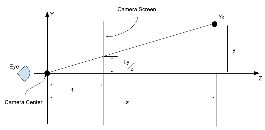
By similar triangles, we have:

\[\frac{y_V}{y}=\frac{f}{z} \\ y_V = \frac{f}{z} y\]

Similarly, we have: \(\displaystyle x_V = \frac{f}{z} x\). Finally, we have the translation from the camera viewfinder to the screen where we will see the image. The mapping to the screen is a simple \(x-y\) translation represented by \(p_x\) and \(p_y\).

Screen Camera Translation

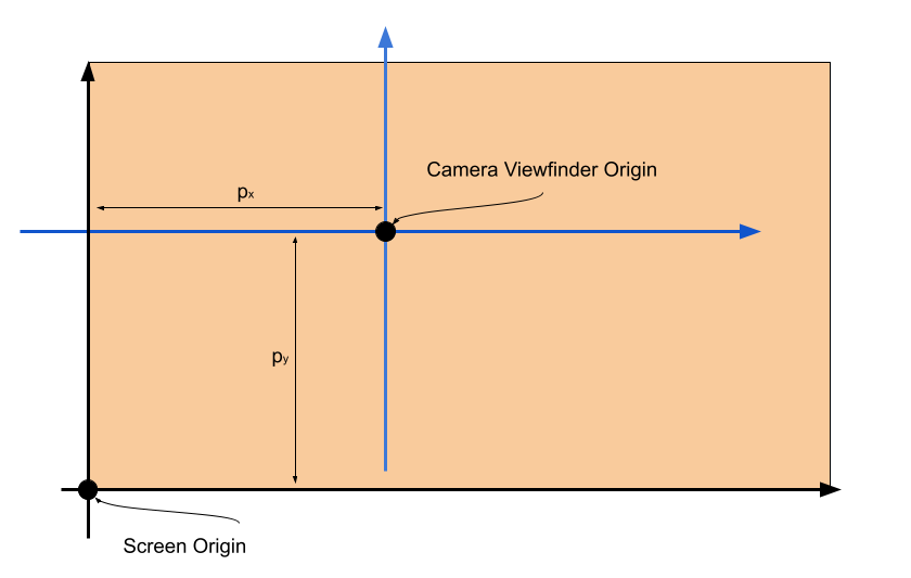
The transform matrix in homogeneous coordinates is thus:

\[\begin{equation} P= \begin{bmatrix} f && 0 && p_x && 0 \\ 0 && f && p_y && 0 \\ 0 && 0 && 1 && 0 \end{bmatrix} \label{eq:3} \end{equation}\]

Note that the above matrix is \(3 \times 4\): passing a 3D coordinate in homogeneous form (\(4 \times 1\)) will yield a \(3 \times 1\) vector.

The result of the transform \(PX_C\) gives us:

\[PX_C = \begin{bmatrix} f && 0 && p_x && 0 \\ 0 && f && p_y && 0 \\ 0 && 0 && 1 && 0 \end{bmatrix} \begin{bmatrix} x_C \\ y_C \\ z_C \\ 1 \end{bmatrix} = \begin{bmatrix} fx_C + z_C p_x \\ fy_C + z_C p_y \\ z_C \\ \end{bmatrix}\]

Since \(z\) is not constant, whatever result we get will be divided throughout by \(z\), to give us the 2D view screen coordinates in homogeneous form.

\[PX_C=\begin{bmatrix} \displaystyle\frac{f}{z}x_C + p_x \\ \displaystyle\frac{f}{z}y_C + p_y \\ 1 \\ \end{bmatrix}\]

Pulling in \(\eqref{eq:2}\), \(\eqref{eq:3}\), and substituting in \(\eqref{eq:3}\), we get:

\[X_V = PB^{-1} (X_W - C)\]

Technical Note: In the actual implementation, the camera center translation is implemented using homogeneous coordinates, so that instead of subtracting the camera center (\(C=(C_x, C_y, C_z)\)), we perform a matrix multiplication, like so:

\[X_V = PB^{-1}.C'.X_W\]

where \(C'=\begin{bmatrix} 0 && 0 && 0 && -C_x \\ 0 && 1 && 0 && -C_y \\ 0 && 0 && 0 && -C_z \\ 0 && 0 && 0 && 1 \end{bmatrix}\).

Implementation

The following code plays around with the pinhole camera model and sets up a very basic (maybe even contrived) volumetric rendering model. The details of the toy volumetric raycasting logic is explained after the listing. The code is annotated with comments so you should be able to follow along.

import math
import numpy as np
import torch
import matplotlib.pyplot as plt


class Camera:
    def __init__(self, focal_length, center, basis):
        camera_center = center.detach().clone()
        transposed_basis = torch.transpose(basis, 0, 1)
        camera_center[:3] = camera_center[
                            :3] * -1  # We don't want to multiply the homogenous coordinate component; it needs to remain 1
        camera_origin_translation = torch.eye(4, 4)
        camera_origin_translation[:, 3] = camera_center
        extrinsic_camera_parameters = torch.matmul(torch.inverse(transposed_basis), camera_origin_translation)
        intrinsic_camera_parameters = torch.tensor([[focal_length, 0., 0., 0.],
                                                    [0., focal_length, 0., 0.],
                                                    [0., 0., 1., 0.]])
        self.transform = torch.matmul(intrinsic_camera_parameters, extrinsic_camera_parameters)

    def to_2D(self, point):
        rendered_point = torch.matmul(self.transform, torch.transpose(point, 0, 1))
        point_z = rendered_point[2, 0]
        return rendered_point / point_z


def camera_basis_from(camera_depth_z_vector):
    depth_vector = camera_depth_z_vector[:3]  # We just want the inhomogenous parts of the coordinates

    # This calculates the projection of the world z-axis onto the surface defined by the camera direction,
    # since we want to derive the coordinate system of the camera to be orthogonal without having
    # to calculate it manually.
    cartesian_z_vector = torch.tensor([0., 0., 1.])
    cartesian_z_projection_lambda = torch.dot(depth_vector, cartesian_z_vector) / torch.dot(
        depth_vector, depth_vector)
    camera_up_vector = cartesian_z_vector - cartesian_z_projection_lambda * depth_vector

    # The camera coordinate system now has the direction of camera and the up direction of the camera.
    # We need to find the third vector which needs to be orthogonal to both the previous vectors.
    # Taking the cross product of these vectors gives us this third component
    camera_x_vector = torch.linalg.cross(depth_vector, camera_up_vector)
    inhomogeneous_basis = torch.stack([camera_x_vector, camera_up_vector, depth_vector, torch.tensor([0., 0., 0.])])
    homogeneous_basis = torch.hstack((inhomogeneous_basis, torch.tensor([[0.], [0.], [0.], [1.]])))
    homogeneous_basis[0] = unit_vector(homogeneous_basis[0])
    homogeneous_basis[1] = unit_vector(homogeneous_basis[1])
    homogeneous_basis[2] = unit_vector(homogeneous_basis[2])
    return homogeneous_basis


def basis_from_depth(look_at, camera_center):
    depth_vector = torch.sub(look_at, camera_center)
    depth_vector[3] = 1.
    return camera_basis_from(depth_vector)


def unit_vector(camera_basis_vector):
    return camera_basis_vector / math.sqrt(
        pow(camera_basis_vector[0], 2) +
        pow(camera_basis_vector[1], 2) +
        pow(camera_basis_vector[2], 2))


def plot(style="bo"):
    return lambda p: plt.plot(p[0][0], p[1][0], style)


def line(marker="o"):
    return lambda p1, p2: plt.plot([p1[0][0], p2[0][0]], [p1[1][0], p2[1][0]], marker="o")


look_at = torch.tensor([0., 0., 0., 1])
camera_center = torch.tensor([-5., -10., 20., 1.])
focal_length = 1.

camera_basis = basis_from_depth(look_at, camera_center)
camera = Camera(focal_length, camera_center, camera_basis)

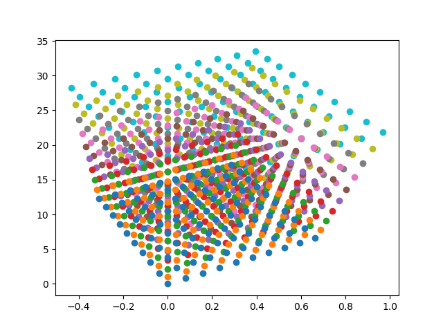
fig1 = plt.figure()

for i in range(10):
    for j in range(10):
        for k in range(10):
            d = camera.to_2D(torch.tensor([[i, j, k, 1.]]))
            print(d)
            plt.plot(d[0][0], d[1][0], marker="o")

ray_origin = camera_center
camera_basis_x = camera_basis[0][:3]
camera_basis_y = camera_basis[1][:3]

unit_vector_x_camera_basis = unit_vector(camera_basis_x)
unit_vector_y_camera_basis = unit_vector(camera_basis_y)

print(unit_vector_x_camera_basis)
print(unit_vector_y_camera_basis)

camera_center_inhomogenous = camera_center[:3]

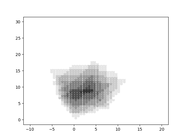
fig2 = plt.figure()

for i in np.linspace(-10, 20, 50):
    for j in np.linspace(0, 30, 50):
        ray_screen_intersection = unit_vector_x_camera_basis * i + unit_vector_y_camera_basis * j
        unit_ray = unit_vector(ray_screen_intersection - camera_center_inhomogenous)
        density = 0.
        for k in np.linspace(0, 100):
            ray_endpoint = camera_center_inhomogenous + unit_ray * k
            ray_x, ray_y, ray_z = ray_endpoint
            if (ray_x < 0 or ray_x > 10 or
                    ray_y < 0 or ray_y > 10 or
                    ray_z < 0 or ray_z > 10):
                continue
            # We are in the box
            density += 0.1
        plt.plot(i, j, marker="o", color=str(1. - density))

plt.show()

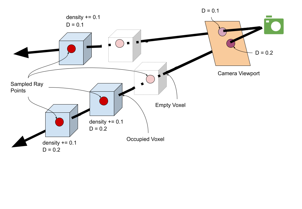
We have not discussed the optical model for volumetric rendering, so for the moment, we will describe a very cheap way of getting a sense of what a volumetric rendering might look like.

Determine a bundle of rays originating from the camera center. These rays will be intersecting the camera viewport.
For each ray, sample a number of points along this ray upto some reasonable limit. The initial “density” of this ray is 0.
For each such point, determine if it lies in an occupied voxel. If it does, increment the density of this ray by a tiny amount.
At the end of the sampling of this ray, the accumulated density will be the greyscale intensity of the pixel in the camera viewport.

We have used a simple \(10 \times 10 \times 10\) cube for this example. There is currently no data structure holding the cube information: we simply assume the cube extends from \((0,0,0)\) upto \((10,0,0)\), \((0,10,0)\), and \((0,0,10)\), and implement the voxel check accordingly.

Basic Volumetric Raycasting

Outputs

This is the voxel image of the cube. Voxel Cube

This is the volumetric render of the cube. As expected, the direction of the diagonal (as seen from the camera) is the densest, as the rays have to pass through the most number of voxels.

Very Basic Volumetric Rendering of Cube

This concludes the first part of building the very basic infrastructure to support building the rest of the paper.

References

tags: Machine Learning - PyTorch - Programming - Neural Radiance Fields - Machine Vision

Total Internal Reflection

Code

Contact