Plenoxels and Neural Radiance Fields using PyTorch: Part 5

Avishek Sen Gupta on 19 December 2022

This is part of a series of posts breaking down the paper Plenoxels: Radiance Fields without Neural Networks, and providing (hopefully) well-annotated source code to aid in understanding.

The final code has been moved to its own repository at plenoxels-pytorch.

We continue looking at Plenoxels: Radiance Fields without Neural Networks. We have built our volumetric renderer, trained it on a single training image; it is now time to extend the idea to multiple training images obtained by cameras around the model. We will also add Total Variance regularisation to the loss calculations in this post, and compare the results for good and skewed initial randomised values. Ultimately, we show results of the reconstruction using our simple cube.

The code for this article can be found here: Volumetric Rendering Code with TV Regularisation

We start off with an explanation of Total Variance Denoising.

Total Variation Denoising

1. One-Dimensional Signal

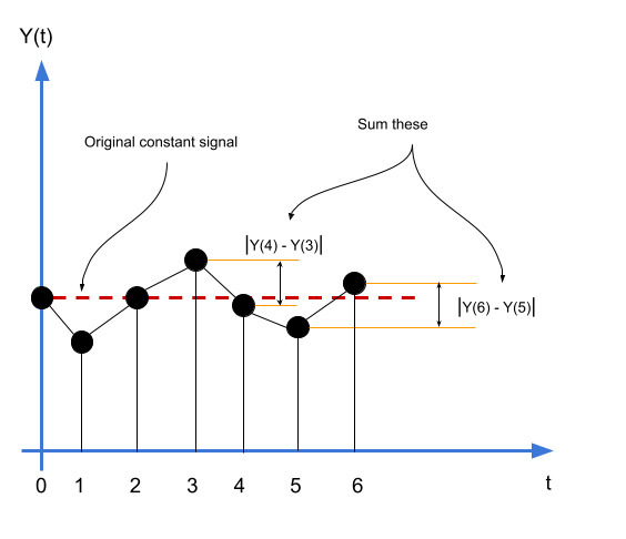
Assume we have a one-dimensional constant signal \(Y(t)\) filled with noise. Since this noise varies from sample to sample, there is always going to be (with a high probability) a difference between consecutive samples of this noisy signal. Our task is to rederive the original constant signal from this noisy signal. We need to minimise the gradient across all samples. In this case, the gradient between two consecutive samples is simply the magnitude of their differences. Thus, define this gradient between \(Y(t+1)\) and \(Y(t)\) as:

\[\delta(t+1) = |Y(t+1) - Y(t)|\]

Then, the total variation of the signal \(\Delta(X)\) is defined as:

\[\begin{equation} {\Delta}_{TV}(Y) = \sum_{t=0}^{T-1} |Y(t+1) - Y(t)| \label{eq:total-variation-1d} \end{equation}\]

The \(T-1\) term is because \(t \in [0, T]\). We need to minimise the cost function \(\Delta(Y)\).

Let us define the problem more precisely. We have some function \(Y = f(X)\), where \(X\) is the original noisy signal, and \(Y\) is the reconstructed signal. We need the total variation of \(Y\) to be the smallest it possibly can be.

Total Variation for One-Dimensional Signal

The above is the extreme case. Normally, signals will not be constant. In that case, simply minimising \({\Delta}_{TV}(Y)\) will always result in a constant signal, which is obviously not desirable. We still need to have the denoised signal look somewhat like the original noisy signal, while minimising the total variation. This similarity can be measured using the mean squared error, like so:

\[\begin{equation} {\Delta}_{MSE}(X,Y) = \frac{1}{T}\sum_0^T {[Y(t) - X(t)]}^2 \label{eq:mse-1d} \end{equation}\]

Thus, we want to minimise the cost function above as well. Putting \(\eqref{eq:total-variation-1d}\) and \(\eqref{eq:mse-1d}\) together, we get:

\[\begin{equation} \Delta(X,Y) = {\Delta}_{MSE}(X,Y) + \lambda {\Delta}_{TV}(Y) \\ \label{eq:full-cost-with-tv} \end{equation} \Delta(X,Y) = \frac{1}{T}\displaystyle\sum_0^T {\bigg[Y(t) - X(t)\bigg]}^2 + \lambda \sum_{t=0}^{T-1} \bigg\lvert Y(t+1) - Y(t) \bigg\rvert\]

where \(\lambda\) is the regularisation parameter, and controls the amount of denoising.

2. Two-Dimensional Signal

Moving to the two-dimensional case, we can extend Total Variation measure to be very similar to mean squared error:

\[\begin{equation} {\Delta}_{TV}(Y) = \sum_{i,j}^{I,J} \sqrt{ {\bigg[Y(i+1, j) - Y(i, j)\bigg]}^2 + {\bigg[Y(i, j+1) - Y(i, j)\bigg]}^2 } \label{eq:total-variation-2d} \end{equation}\]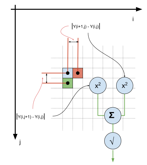

Total Variation for Two-Dimensional Signal

The overall cost function remains to be \(\Delta(X,Y) = {\Delta}_{MSE}(X,Y) + \lambda {\Delta}_{MSE}(Y)\).

3. Application to Plenoxels

We are now ready to apply TV denoising to our problem. As it turns out, we use the exact same cost function with the following ideas:

The cost function is extended to three dimensions similar to how we framed the problem in two dimensions.
The cost function is applied independently to each of our 28 dimensions (1 opacity, 27 spherical harmonic coefficients)

Assume the voxels are in the set \(V\), the TV regularisation term then is:

\[{\Delta}_{TV} = \frac{1}{|V|}\sum_{i,j \in V, d \in D} \sqrt{ {\bigg[Y_d(i+1, j, k) - Y_d(i, j, k)\bigg]}^2 + {\bigg[Y_d(i, j+1, k) - Y_d(i, j, k)\bigg]}^2 + {\bigg[Y_d(i, j, k+1) - Y_d(i, j, k)\bigg]}^2 }\]

which is simply written in the paper as:

\[{\Delta}_{TV} = \frac{1}{|V|}\sum_{i,j \in V, d \in D} \sqrt{ \delta_i^2 + \delta_j^2 + \delta_k^2 }\]

where

\[\delta_i = \bigg\lvert Y_d(i+1, j, k) - Y_d(i, j, k) \bigg\rvert \\ \delta_j = \bigg\lvert Y_d(i, j+1, k) - Y_d(i, j, k) \bigg\rvert \\ \delta_k = \bigg\lvert Y_d(i, j, k+1) - Y_d(i, j, k) \bigg\rvert\]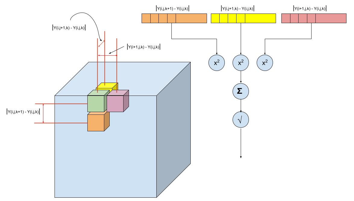

Total Variation for Three-Dimensional Signal

The final cost function in the paper is then exactly the same as we described above in \(\eqref{eq:full-cost-with-tv}\):

\[\Delta(X,Y) = {\Delta}_{MSE}(X,Y) + \lambda {\Delta}_{MSE}(Y)\]

where, \(X\) is our training image.

Constructing model parameters differently

We now modify the code to handle multiple training images. So far, we have been recreating a new PlenoxelModel instance for every training cycle. The reason is that the parameters to optimise vary per cycle, depending upon which stochastic sample of rays we select. The recommended way to vary parameters in a model is to mark a subset of the parameters we want to freeze, as requires_grad=False, and this is what we do. All the voxels in the world are considered as parameters by default. For each training scene, we decide which voxels intersect with our viewing rays, and mark those as requiring gradient propagation. We simply set requires_grad=True for the voxels which should be considered for updates, and set it to False for the others. See modify_grad() for how this done.

Notes on the Reconstruction

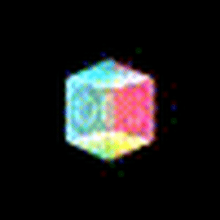
Initial values are important. Random values of the spherical harmonic coefficients were initially between 0 and 1. That gave the reconstruction below. From certain angles, the reconstruction does not look like a cube, or only partially like one.

The pictures below compare the reconstruction with the actual ground truth, when the initial values are skewed to be only positive.

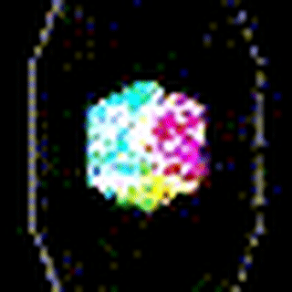
Crude Reconstruction of Cube Original Cube

Changing the initial random values to between -1 and 1, gives us the following, much improved reconstructions:

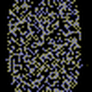
Cube Reconstruction using good initial values Original Cube

These are training scenes from the first three epochs:

Cube Reconstruction training steps

More epochs and training images are obviously needed. The paper mentions running 12800 batches before it converges sufficiently.

Parallelising Volumetric Calculations using PyTorch

One of the issues faced with the current code is that it is very slow. A single training image, which includes calculation of the intersecting voxels, loss calculations, and the single optimisation step, takes about 42 seconds. The paper implements a CUDA-based volumetric renderer, and this is an interesting project we might consider tackling at some point from scratch. We could have either used Pathos or PyTorch’s multiprocessing library. Unfortunately, PyTorch cannot perform distributed gradient propagation (there is an experimental feature for it, but we haven’t tried it), so we ended up using Pathos. It will probably more effective if the volumetric calculations are more intensive; currently, the distributed version takes longer than the serial version.

Look at render_parallel() to see how Pathos is used.

Debugging Out of Memory issues

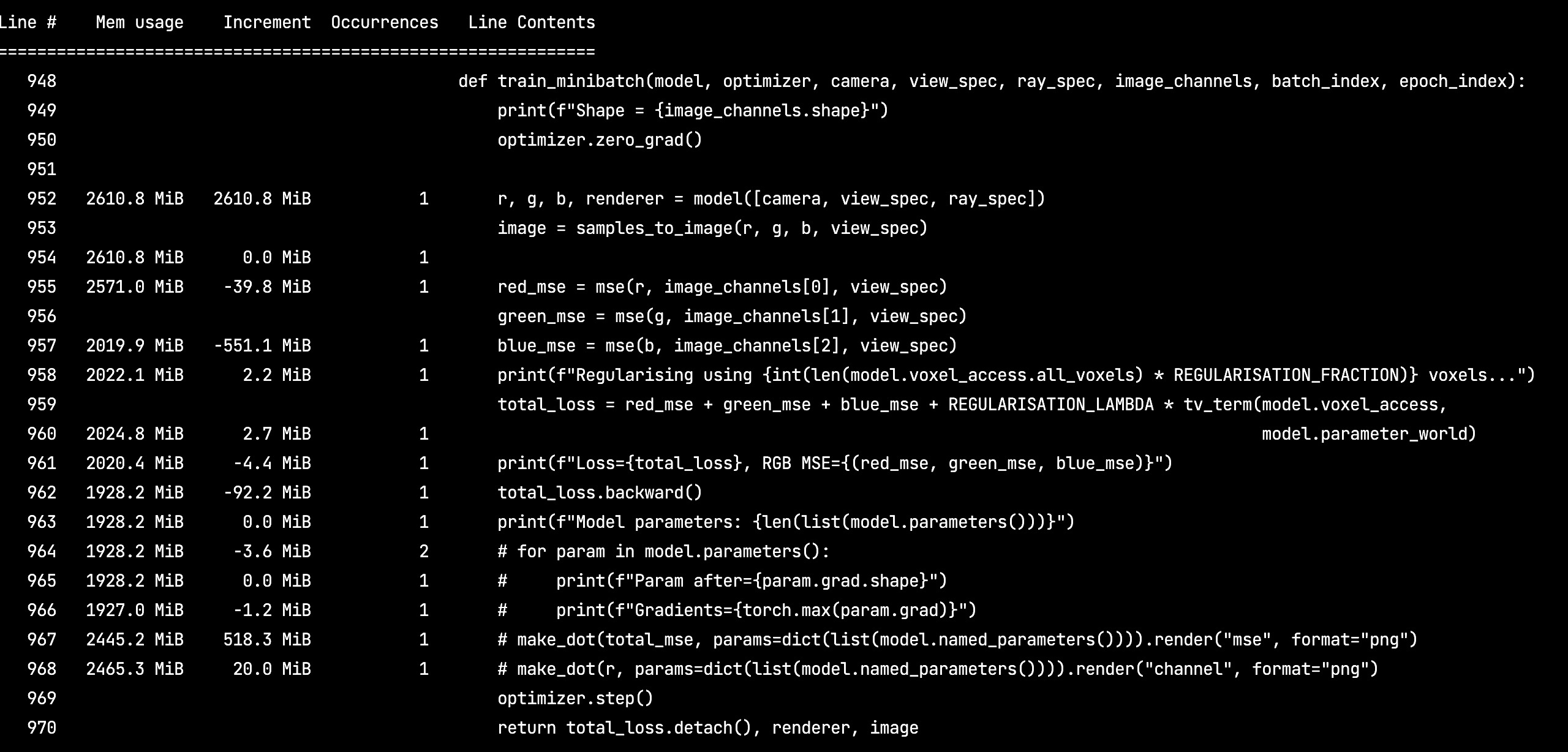
One of the issues we faced was accidentally retaining the entire computational graph after each loss calculation. Appending losses to an array as-is, retains a reference to the graph, which can continue holding more than 1 GB of memory, causing the OS to terminate the Python process somewhere in the 3rd epoch.

Memory Profiler makes it very easy to track incremental per-line memory allocation, and track down such issues.

Here is an example screenshot of the library output running:

memory-profiler output

Furthermore, user ptrblck says this:

“If you are seeing an increased memory usage of 10GB in each iteration, you are most likely storing the computation graph accidentally by e.g. appending the loss (without detaching it) to a list etc.”

Conclusion

We have incorporated Total Variance regularisation in our implementation of the paper, and implemented a proper training schedule using multiple training images. The reconstructions are crude, but they demonstrate how the spherical harmonics can be learned and varied from different angles. There are a few more details that we will need to address in a sequel, specifically:

Voxel pruning: This will probably require us to modify our core data structure to be a little more efficient, because it will involve storing all the transmittances of the entire training set per epoch, and then zeroing out candidate voxels.
Encouraging voxel sparsity: Adding more regularisation terms will encourage sparsity of voxels. In the paper, the Cauchy loss is incorporated to speed up computations.
Coarse-to-fine resolution scaling: This will be needed to better resolve the fine structure of our training scenes. At this point, we are working with a very coarse low resolution of \(40 \times 40 \times 40\). We can get higher resolutions than this, but this will need more work, and more computations.

References

tags: Machine Learning - PyTorch - Programming - Neural Radiance Fields - Machine Vision

Total Internal Reflection

Code

Contact